Linear regression is a special case of generalized linear modeling that seeks to minimize the mean squared error on a continuous spectrum between each all datapoints in the dataset and the predicted output value. It makes an assumption that the underlying data can be modeled using a weighted linear combination of sums:
\[
\hat{y}=w_1x_1+w_2x_2+...+w_kx_k + b
\tag{9.1}\]
The optimization function is the mean squared error, or the distance between each datapoint in the dataset and the prediction line:
The act of identifying the weights allows a user to make a prediction on the interval \((-\infty,\infty)\) to make a numeric prediction for an output or dependent variable \(Y\), based upon a vector of input \(X\).
9.1.2 Logistic Regression
9.1.2.1 What is Logistic Regression?
Logistic regression is a method to predict a probability of a boolean outcome on the interval from \([0,1]\). To perform this action, logistic regression uses linear regression in combination with the sigmoid function \(\hat{y}=\frac{1}{1+e^{-z}}\) where \(z = w_1x_1+w_2x_2+...+w_kx_k + b\), and gradient ascent (or descent, depending on implementation), to link the linear equation from all real numbers to the interval [0,1].
9.1.2.2 How do Logistic and Linear Regression Compare?
The key similarity between linear and logisitic regression is the use of a linear combination of weighted sums as in Equation 9.1 above, and each leverage an optimization problem to maximize performance of their predictive outcomes. However, this is about where their similarities end. The difference in the output space (\((-\infty,\infty)\) vs \([0,1]\)), the type of optimization problem used (mean squared error minimization vs. maximum likelihood estimation), and their applications (continuous numeric prediction vs. probability prediction), truly set these two regression methods apart.
9.1.2.3 How Does Logistic Regression Predict Probability?
The sigmoid function is paramount in the implementation of logisitic regression as it remaps the output space of a linear regression to have limited bounds on the interval \([0,1]\). Since linear regression has an infinite output space, it is less useful in the prediction of an outcome or a class. The sigmoid function, and derivations from it, are used to train logistic regression models and to make predictions with them once they are trained.
9.1.2.4 How is Logistic Regression Trained?
Maximum likelihood estimation is used as part of the optimization effort for a logisitic regression. Each weight \(w_i\) in the equation for \(z\) above needs to be adapted and adjusted so as to maximize the likelihood that the input dataset is correctly classified. To calculate the change in probability, the algorithm leverages partial derivatives to calculate how each weight should be adjusted while pursuing a local maximum (gradient ascent) or minimum (gradient descent) using
the log likelihood function \[
\text{log(p(y|x)} = \sum\limits_{i=1}^ny_i\cdot \text{log}(\hat{y}_i)+(1-y_i)\cdot\text{log}(1-\hat{y}_i)
\tag{9.3}\]
partial derivatives of the likelihood with respect to each feature \[
\frac{\delta L}{\delta w_i} = (\hat{y_i}-y_i)x_i = \frac{\delta L}{\delta \hat{y}_i}\frac{\delta\hat{y}_i}{\delta z}\frac{\delta z}{\delta w_i}
\tag{9.4}\]
to iteratively move the needle in the right direction.
9.1.2.5 How Is Maximum Likelihood Used in Logisitic Regression?
Using the above, each iteration of a logistic regression seeks to increase the likelihood, or probability to that a given input vector \(X\) will be classified as the appropriate category \(Y\) by adjusting the weights to bring the output probability closer to zero when \(X\) is not a member of \(Y\), and closer to 1 when \(X\) is a member of \(Y\). This method can enter the pitfall of solely achieving a local minimum or maximum vs. a global minimum or maximum, as one cannot directly know or infer a parametric equation for \(\text{log(p(y|x))}\).
9.2 Data
The data used for logistic regression is output from the multiple correspondence analysis (MCA) section. The code will leverage two outputs - the MCA that includes the protected classes, and the MCA that does not.
The process to generate these data is contained and described in Appendix G.
As done in Chapter 7 for train test splits - the indexes are disjoint between training and testing datasets for each parent dataset (with and without protected classes), and each model is trained with the same records for comparison and evaluation against one another (same records for training and testing allow for direct comparison of the models).
By achieving these splits, the two models evaluated with and without protected class information will avoid unnecessary biases in the results. When a model is tested on data with which it has already been trained, the model has already optimized to the best of its ability to correctly classify the training data. As such, the outcome of an evaluation of a model using the same data in training and testing will artificially inflate its performance metrics (accuracy, precision, recall, F1, ROC-AUC). As such, it is paramount to have a disjoint training and testing dataset.
Here are the first few rows of the training and testing data (excluding protected classes):
Table 9.1: MCA Training Data (With Protected Classes)
MC1
MC2
MC3
MC4
MC5
MC6
MC7
MC8
MC9
MC10
...
MC173
MC174
MC175
MC176
MC177
MC178
MC179
MC180
MC181
outcome
149746
-0.387299
-0.001936
-0.003167
-0.003736
-0.024160
-0.058848
-0.161641
-0.163059
0.051339
-0.009136
...
0.003101
-0.001341
0.000861
0.004199
-0.000527
-0.002532
-0.008719
-0.000873
-0.002317
1.0
105015
-0.386534
0.007586
0.005638
-0.149832
0.037838
0.251784
0.098772
-0.104072
0.013961
-0.418258
...
0.000377
0.001873
0.001106
-0.027093
0.005149
0.003389
0.007496
-0.003416
0.003757
1.0
29094
0.584290
-0.011996
-0.005619
0.162373
-0.135637
-0.251829
-0.104188
-0.168750
-0.177008
0.118405
...
0.022515
-0.007842
-0.002415
-0.049875
0.001095
0.072832
-0.005292
0.078073
0.014257
1.0
101082
-0.334664
0.002222
0.000164
-0.101558
0.021665
-0.211819
0.279624
0.695377
0.687991
-0.076981
...
0.026285
0.001354
-0.002768
0.006803
0.007875
0.004828
0.006313
-0.007748
0.009507
1.0
77750
-0.281561
0.009739
0.007302
0.294964
-0.119251
0.159063
0.758784
-0.039995
-0.195625
0.002697
...
-0.052733
-0.000610
-0.008253
0.117513
0.000083
0.007967
-0.010744
-0.000727
0.000273
1.0
197336
0.486499
-0.010249
-0.000090
-0.015523
-0.006435
0.167655
-0.198908
0.150687
-0.162005
0.046811
...
-0.012404
-0.000997
-0.002124
0.001909
0.000212
-0.007067
0.015649
0.006640
-0.000096
0.0
137650
0.467874
0.001350
-0.009676
-1.188243
0.363408
0.128250
0.223274
-0.317145
0.196431
-0.287222
...
-0.019506
-0.000767
-0.000612
-0.005116
0.001205
-0.005075
0.000100
-0.000287
-0.002095
1.0
136772
-0.367590
-0.001345
-0.000256
-0.156002
0.020358
-0.132456
0.018576
-0.093998
0.103849
0.001622
...
-0.106859
0.004671
0.000376
0.009465
-0.000201
0.007182
-0.011129
-0.008761
-0.001996
1.0
41734
-0.330008
0.011018
0.006242
0.272821
-0.054578
0.325838
0.372732
0.030138
-0.028335
0.063026
...
0.011053
0.001163
0.004312
-0.062842
0.000968
0.007450
-0.009850
-0.003101
0.003397
0.0
10710
-0.426415
-0.004343
-0.003192
0.108570
-0.054307
-0.125460
-0.280849
0.185723
-0.081365
0.132101
...
0.020289
-0.005505
0.000400
0.092377
0.001436
0.006528
-0.011197
0.000699
-0.019417
1.0
10 rows × 182 columns
Table 9.2: MCA Testing Data (With Protected Classes)
MC1
MC2
MC3
MC4
MC5
MC6
MC7
MC8
MC9
MC10
...
MC173
MC174
MC175
MC176
MC177
MC178
MC179
MC180
MC181
outcome
30860
-0.377629
-0.003778
-0.000284
0.123173
-0.082610
-0.252011
-0.083817
0.137802
-0.059589
0.146982
...
0.033447
-0.004992
0.012373
-0.043422
-0.000974
0.003553
0.006232
0.001033
-0.018414
1.0
126890
-0.467556
0.004930
-0.005359
-0.641571
0.206492
0.242741
-0.226606
-0.014591
-0.472724
0.021588
...
0.010695
-0.000696
0.000022
0.016918
0.003402
-0.003975
-0.003803
0.001092
-0.000510
1.0
28730
-0.413508
-0.005233
0.001155
0.121581
-0.085867
-0.230894
-0.106145
0.189636
-0.061267
0.069930
...
0.015688
0.000374
-0.005150
-0.031315
-0.003929
0.005044
0.008720
0.012316
-0.079917
1.0
31244
-0.287660
-0.003570
0.003981
0.050584
-0.079588
-0.564932
0.493067
0.565763
0.294100
0.394073
...
0.071348
0.005973
0.002630
-0.031388
0.001923
-0.059667
0.008618
0.053812
0.008861
1.0
56105
0.475915
0.012787
-0.010241
0.304675
-0.048947
0.467680
-0.300472
-0.138536
0.078400
0.050529
...
0.021655
-0.007473
0.009129
-0.029546
0.005734
-0.003265
-0.093248
0.005869
-0.020469
1.0
5443
-0.532447
-0.000680
-0.000100
0.149901
-0.052502
0.037784
-0.165450
0.385730
-0.450069
0.097568
...
-0.175609
0.002486
0.005582
-0.060549
-0.006316
-0.007500
0.009540
0.004287
0.003089
1.0
95702
0.488661
0.002546
0.001658
0.293300
-0.075460
0.567510
-0.399183
0.208255
0.236614
-0.575200
...
0.051268
-0.003152
-0.000812
0.022663
-0.002750
-0.011304
0.013903
0.001937
0.017053
1.0
83812
0.618010
-0.008268
0.003282
0.208434
-0.083836
0.068062
0.195019
0.212166
0.059184
-0.127586
...
-0.056974
-0.001156
-0.027070
0.117950
0.000061
0.008795
-0.008416
0.003242
-0.017692
0.0
84338
0.655969
-0.004918
-0.006596
0.294970
-0.113992
0.117014
-0.038303
-0.000417
0.119094
-0.173938
...
-0.025098
-0.003851
-0.015221
0.000430
0.005239
0.005173
-0.009246
0.003599
-0.017117
1.0
124545
0.570068
-0.019301
-0.010219
0.132395
-0.125488
-0.262735
0.254719
-0.193122
-0.455048
0.200752
...
0.018821
0.002103
0.000520
0.011330
-0.000257
0.012774
0.019057
0.005942
0.000166
1.0
10 rows × 182 columns
Table 9.3: MCA Training Data (Without Protected Classes)
MC1
MC2
MC3
MC4
MC5
MC6
MC7
MC8
MC9
MC10
...
MC92
MC93
MC94
MC95
MC96
MC97
MC98
MC99
MC100
outcome
149746
-0.022191
-0.265491
-0.089926
0.030741
-0.203565
0.045974
0.036976
-0.158538
-0.089747
-0.118819
...
0.018080
-0.010963
-0.029876
-0.003884
-0.001979
0.007441
-0.007867
0.005483
-0.000806
1.0
105015
0.290036
0.178485
-0.157600
-0.271749
-0.245192
0.415834
0.123361
0.055042
-0.280792
-0.105106
...
0.032420
0.008380
-0.046675
-0.011824
0.044305
0.096120
0.266568
0.009842
0.006172
1.0
29094
-0.095327
-0.086033
-0.071726
-0.077756
-0.175656
-0.205904
-0.027044
-0.228361
-0.037807
-0.112685
...
0.011820
-0.023923
0.035317
0.019936
-0.090864
0.017211
0.003241
-0.006380
-0.000049
1.0
101082
-0.654622
0.371221
0.433967
0.351343
0.378372
1.075594
-0.389695
-0.187974
-0.091264
-0.120999
...
-0.048364
0.117014
-0.080124
0.017038
0.005769
0.113322
0.239627
0.041617
0.008369
1.0
77750
-0.011772
0.645262
0.057628
-0.176639
-0.285778
-0.331408
-0.273163
0.149750
-0.234999
0.106382
...
0.236344
-0.074790
-0.100306
-0.338227
-0.034114
0.028328
-0.038353
-0.014300
0.001131
1.0
197336
0.211278
-0.030244
0.227029
-0.003941
0.369867
-0.046471
0.319009
-0.191355
-0.301365
0.207057
...
0.031491
-0.015596
-0.012795
-0.014921
-0.018947
0.004192
-0.022371
0.006839
-0.000022
0.0
137650
-0.358538
0.051337
-0.836959
-0.183025
0.827005
-0.153045
-0.300371
0.067741
-0.113371
-0.321046
...
0.335969
-0.153317
0.006543
0.153396
0.313536
-0.124046
0.047060
-0.003220
0.003096
1.0
136772
-0.224883
-0.192682
-0.084809
0.117577
-0.313160
-0.083558
0.224909
0.148168
-0.065917
-0.105496
...
0.182218
0.384711
0.246450
-0.027070
-0.039627
-0.072453
0.029784
-0.224192
-0.000603
1.0
41734
0.126939
0.621233
0.144349
0.053672
-0.309407
-0.342110
-0.120858
0.063892
-0.205557
-0.164335
...
0.072717
-0.012892
-0.102817
-0.445682
-0.024483
0.166019
-0.124861
-0.005165
0.002151
0.0
10710
0.163013
-0.275794
0.117153
-0.011200
-0.019967
0.048655
0.044069
-0.165311
0.018394
-0.103244
...
-0.030015
0.019834
-0.002256
-0.022811
0.042606
-0.007783
-0.012869
-0.010702
-0.000356
1.0
10 rows × 101 columns
Table 9.4: MCA Testing Data (Without Protected Classes)
MC1
MC2
MC3
MC4
MC5
MC6
MC7
MC8
MC9
MC10
...
MC92
MC93
MC94
MC95
MC96
MC97
MC98
MC99
MC100
outcome
30860
0.021908
-0.107937
0.160667
-0.096196
0.018201
-0.101238
0.033902
-0.304192
0.099209
-0.167334
...
-0.041614
0.049508
0.024640
0.119880
0.038063
-0.152665
0.053603
-0.017657
-0.001590
1.0
126890
0.480633
-0.445114
0.321141
-0.039117
0.011562
-0.032186
-0.610614
0.551665
0.076726
0.035808
...
-0.031216
0.024834
-0.065209
-0.075517
0.059589
-0.056023
0.004988
0.007007
0.003624
1.0
28730
-0.008824
-0.143329
0.122037
-0.081711
0.180048
-0.110025
0.093520
-0.358804
0.058229
-0.195015
...
-0.070911
0.049980
-0.013948
-0.019076
0.031768
-0.006892
-0.030458
-0.016992
-0.001599
1.0
31244
-0.929934
0.290919
0.916922
0.393976
0.653189
0.575340
-0.367097
-0.433499
-0.010454
0.096068
...
0.139571
0.046301
-0.099484
-0.084230
-0.004915
0.071326
-0.032964
0.019019
0.000421
1.0
56105
0.414472
0.449156
-0.207480
-0.003224
-0.150305
0.032234
-0.191760
0.153439
1.021892
-0.041131
...
-0.055936
0.036294
0.038325
0.232323
0.003879
0.034577
0.006583
0.002948
0.006281
1.0
5443
0.523671
-0.283900
0.655485
-0.123366
0.718045
-0.163190
-0.157075
0.188473
0.113406
0.062999
...
-0.058962
0.001311
0.019947
-0.076058
-0.048344
-0.037792
-0.004104
-0.015193
-0.001536
1.0
95702
0.473073
0.236969
-0.363466
-0.336683
-0.106912
1.000458
0.259367
0.206744
-0.271422
0.230963
...
-0.101931
0.052594
-0.061589
0.005126
-0.186917
-0.079407
-0.302814
-0.002668
-0.006435
1.0
83812
-0.140662
0.424349
0.083509
-0.163135
-0.410733
-0.206931
-0.126389
-0.014700
-0.278051
-0.149923
...
0.003635
0.030724
-0.095295
-0.276234
0.016694
0.262435
-0.092800
-0.011479
0.001361
0.0
84338
0.060723
0.581497
-0.263134
-0.246079
-0.336327
-0.090347
-0.142133
-0.116463
0.962056
0.254970
...
-0.010415
0.008387
-0.065012
-0.232432
0.236782
0.015017
0.039840
-0.005290
0.007312
1.0
124545
-0.019499
-0.310502
-0.078770
0.035220
-0.240221
0.032627
-0.037473
-0.112962
-0.098873
-0.104411
...
0.036539
-0.009720
-0.027945
-0.016062
0.043209
0.004422
0.017510
0.006984
0.000563
1.0
10 rows × 101 columns
Notice that each has a different number of components. Each is structured to a number of components required to explain at least approximately 99.99% of the variance in each dataset.
Similarly as in Chapter 7 and Chapter 8, a 500 iteration randomization of source data test was performed against both models to compare a difference in means.
9.2.2 Multinomial Naive Bayes
The description for MultinomialNB data and code can be found in Chapter 7.
Table 9.5: Initial Data Used
state_code
county_code
derived_sex
action_taken
purchaser_type
preapproval
open-end_line_of_credit
loan_amount
loan_to_value_ratio
interest_rate
...
tract_median_age_of_housing_units
applicant_race
co-applicant_race
applicant_ethnicity
co-applicant_ethnicity
aus
denial_reason
outcome
company
income_from_median
0
OH
39153.0
Sex Not Available
1
0
2
2
665000.0
85.000
4.250
...
36
32768
131072
32
128
64
512
1.0
JP Morgan
True
1
NY
36061.0
Male
1
0
2
2
755000.0
21.429
4.250
...
0
32768
262144
64
256
64
512
1.0
JP Morgan
False
2
NY
36061.0
Sex Not Available
1
0
1
2
965000.0
80.000
5.250
...
0
65536
262144
64
256
64
512
1.0
JP Morgan
False
3
FL
12011.0
Male
1
0
2
2
705000.0
92.175
5.125
...
12
32768
262144
32
256
64
512
1.0
JP Morgan
False
4
MD
24031.0
Joint
1
0
2
2
1005000.0
65.574
5.625
...
69
66
32768
32
32
64
512
1.0
JP Morgan
False
5
NC
37089.0
Joint
1
0
1
2
695000.0
85.000
6.000
...
39
32768
32768
32
32
64
512
1.0
JP Morgan
False
6
CA
6073.0
Joint
2
0
2
2
905000.0
75.000
6.250
...
44
2
2
32
32
64
512
1.0
JP Morgan
False
7
NY
36061.0
Sex Not Available
2
0
1
2
355000.0
15.909
5.625
...
63
65536
65536
64
64
64
512
1.0
JP Morgan
False
8
NY
36061.0
Joint
1
0
1
2
1085000.0
90.000
5.625
...
75
32768
32768
32
32
64
512
1.0
JP Morgan
True
9
MO
29189.0
Sex Not Available
2
0
1
2
405000.0
53.333
5.750
...
0
65536
65536
64
64
64
512
1.0
JP Morgan
True
10 rows × 51 columns
Table 9.6: MultinomialNB Training Data (With protected classes)
derived_sex_Female
derived_sex_Joint
derived_sex_Male
derived_sex_Sex Not Available
purchaser_type_0
purchaser_type_1
purchaser_type_3
purchaser_type_5
purchaser_type_6
purchaser_type_9
...
co-applicant_ethnicity_No Co-applicant
aus_Desktop Underwriter
aus_Loan Prospector/Product Advisor
aus_TOTAL Scorecard
aus_GUS
aus_Other
aus_Internal Proprietary
aus_Not applicable
aus_Exempt
outcome
149746
1
0
0
0
0
1
0
0
0
0
...
1
1
0
0
0
0
0
0
0
1.0
105015
0
0
1
0
1
0
0
0
0
0
...
1
1
0
0
0
0
0
0
0
1.0
29094
0
1
0
0
0
1
0
0
0
0
...
0
1
1
0
0
1
0
0
0
1.0
101082
0
0
1
0
1
0
0
0
0
0
...
1
1
0
0
0
0
0
0
0
1.0
77750
1
0
0
0
1
0
0
0
0
0
...
1
0
0
0
0
0
1
0
0
1.0
197336
0
1
0
0
1
0
0
0
0
0
...
0
0
1
0
0
0
0
0
0
0.0
137650
0
0
0
1
0
1
0
0
0
0
...
0
1
0
0
0
0
0
0
0
1.0
136772
1
0
0
0
0
1
0
0
0
0
...
1
1
0
0
0
0
0
0
0
1.0
41734
1
0
0
0
1
0
0
0
0
0
...
1
0
1
0
0
0
1
0
0
0.0
10710
1
0
0
0
0
0
1
0
0
0
...
1
0
1
0
0
1
0
0
0
1.0
10 rows × 244 columns
Table 9.7: MultinomialNB Testing Data (With protected classes)
derived_sex_Female
derived_sex_Joint
derived_sex_Male
derived_sex_Sex Not Available
purchaser_type_0
purchaser_type_1
purchaser_type_3
purchaser_type_5
purchaser_type_6
purchaser_type_9
...
co-applicant_ethnicity_No Co-applicant
aus_Desktop Underwriter
aus_Loan Prospector/Product Advisor
aus_TOTAL Scorecard
aus_GUS
aus_Other
aus_Internal Proprietary
aus_Not applicable
aus_Exempt
outcome
30860
0
0
1
0
0
0
1
0
0
0
...
1
1
1
0
0
1
0
0
0
1.0
126890
0
0
0
1
0
0
1
0
0
0
...
1
1
0
0
0
0
0
0
0
1.0
28730
0
0
1
0
0
0
1
0
0
0
...
1
1
1
0
0
1
0
0
0
1.0
31244
0
0
1
0
0
0
1
0
0
0
...
1
1
1
0
0
1
0
0
0
1.0
56105
0
0
1
0
0
0
1
0
0
0
...
0
0
1
0
0
0
0
0
0
1.0
5443
0
0
1
0
0
0
1
0
0
0
...
1
0
1
0
0
0
0
0
0
1.0
95702
0
1
0
0
1
0
0
0
0
0
...
0
0
0
0
0
0
0
1
0
1.0
83812
0
1
0
0
1
0
0
0
0
0
...
0
0
0
0
0
0
1
0
0
0.0
84338
0
1
0
0
0
0
1
0
0
0
...
0
0
1
0
0
0
0
0
0
1.0
124545
0
1
0
0
0
0
1
0
0
0
...
0
1
0
0
0
0
0
0
0
1.0
10 rows × 244 columns
Table 9.8: MultinomialNB Training Data (No protected classes)
purchaser_type_0
purchaser_type_1
purchaser_type_3
purchaser_type_5
purchaser_type_6
purchaser_type_9
purchaser_type_71
preapproval_1
preapproval_2
open-end_line_of_credit_1
...
tract_median_age_of_housing_units_H
tract_median_age_of_housing_units_M
tract_median_age_of_housing_units_MH
tract_median_age_of_housing_units_ML
company_Bank of America
company_JP Morgan
company_Navy Federal Credit Union
company_Rocket Mortgage
company_Wells Fargo
outcome
149746
0.0
1.0
0.0
0.0
0.0
0.0
0.0
0.0
1.0
0.0
...
0.0
1.0
0.0
0.0
0.0
0.0
0.0
1.0
0.0
1.0
105015
1.0
0.0
0.0
0.0
0.0
0.0
0.0
0.0
1.0
0.0
...
0.0
1.0
0.0
0.0
0.0
0.0
1.0
0.0
0.0
1.0
29094
0.0
1.0
0.0
0.0
0.0
0.0
0.0
0.0
1.0
0.0
...
0.0
1.0
0.0
0.0
0.0
1.0
0.0
0.0
0.0
1.0
101082
1.0
0.0
0.0
0.0
0.0
0.0
0.0
0.0
1.0
0.0
...
0.0
0.0
0.0
1.0
0.0
0.0
1.0
0.0
0.0
1.0
77750
1.0
0.0
0.0
0.0
0.0
0.0
0.0
0.0
1.0
0.0
...
0.0
0.0
1.0
0.0
0.0
0.0
0.0
0.0
1.0
1.0
197336
1.0
0.0
0.0
0.0
0.0
0.0
0.0
0.0
1.0
0.0
...
0.0
1.0
0.0
0.0
0.0
0.0
0.0
1.0
0.0
0.0
137650
0.0
1.0
0.0
0.0
0.0
0.0
0.0
0.0
1.0
0.0
...
0.0
0.0
0.0
1.0
0.0
0.0
0.0
1.0
0.0
1.0
136772
0.0
1.0
0.0
0.0
0.0
0.0
0.0
0.0
1.0
0.0
...
0.0
1.0
0.0
0.0
0.0
0.0
0.0
1.0
0.0
1.0
41734
1.0
0.0
0.0
0.0
0.0
0.0
0.0
0.0
1.0
0.0
...
0.0
0.0
1.0
0.0
1.0
0.0
0.0
0.0
0.0
0.0
10710
0.0
0.0
1.0
0.0
0.0
0.0
0.0
0.0
1.0
0.0
...
0.0
1.0
0.0
0.0
0.0
1.0
0.0
0.0
0.0
1.0
10 rows × 176 columns
Table 9.9: MultinomialNB Training Data (No protected classes)
purchaser_type_0
purchaser_type_1
purchaser_type_3
purchaser_type_5
purchaser_type_6
purchaser_type_9
purchaser_type_71
preapproval_1
preapproval_2
open-end_line_of_credit_1
...
tract_median_age_of_housing_units_H
tract_median_age_of_housing_units_M
tract_median_age_of_housing_units_MH
tract_median_age_of_housing_units_ML
company_Bank of America
company_JP Morgan
company_Navy Federal Credit Union
company_Rocket Mortgage
company_Wells Fargo
outcome
30860
0.0
0.0
1.0
0.0
0.0
0.0
0.0
0.0
1.0
0.0
...
0.0
1.0
0.0
0.0
0.0
1.0
0.0
0.0
0.0
1.0
126890
0.0
0.0
1.0
0.0
0.0
0.0
0.0
0.0
1.0
0.0
...
0.0
0.0
1.0
0.0
0.0
0.0
0.0
1.0
0.0
1.0
28730
0.0
0.0
1.0
0.0
0.0
0.0
0.0
0.0
1.0
0.0
...
0.0
0.0
0.0
1.0
0.0
1.0
0.0
0.0
0.0
1.0
31244
0.0
0.0
1.0
0.0
0.0
0.0
0.0
0.0
1.0
0.0
...
0.0
1.0
0.0
0.0
0.0
1.0
0.0
0.0
0.0
1.0
56105
0.0
0.0
1.0
0.0
0.0
0.0
0.0
0.0
1.0
0.0
...
0.0
0.0
0.0
1.0
1.0
0.0
0.0
0.0
0.0
1.0
5443
0.0
0.0
1.0
0.0
0.0
0.0
0.0
0.0
1.0
0.0
...
0.0
0.0
0.0
1.0
0.0
1.0
0.0
0.0
0.0
1.0
95702
1.0
0.0
0.0
0.0
0.0
0.0
0.0
0.0
1.0
0.0
...
0.0
1.0
0.0
0.0
0.0
0.0
1.0
0.0
0.0
1.0
83812
1.0
0.0
0.0
0.0
0.0
0.0
0.0
0.0
1.0
0.0
...
0.0
1.0
0.0
0.0
0.0
0.0
0.0
0.0
1.0
0.0
84338
0.0
0.0
1.0
0.0
0.0
0.0
0.0
0.0
1.0
0.0
...
0.0
1.0
0.0
0.0
0.0
0.0
0.0
0.0
1.0
1.0
124545
0.0
0.0
1.0
0.0
0.0
0.0
0.0
0.0
1.0
0.0
...
0.0
1.0
0.0
0.0
0.0
0.0
0.0
1.0
0.0
1.0
10 rows × 176 columns
9.3 Code
The code for both logistic regression can be found in Appendix F and multinomial naive bayes in Appendix D.
9.4 Results
9.4.1 Logistic Regression
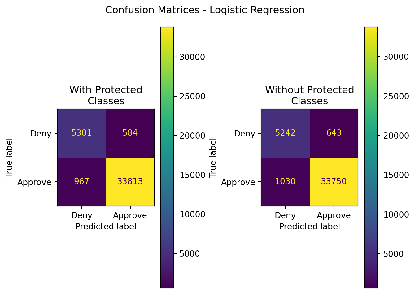
Figure 9.1: Logistic Regression Modeling Results
Table 9.10: Logistic Regression Model Metrics
Model
Data
Accuracy
Precision
Recall
F1
ROC-AUC
Logistic Regression
With Protected Classes
0.961859
0.983022
0.972197
0.977579
0.936481
Logistic Regression
Without Protected Classes
0.958859
0.981304
0.970385
0.975814
0.930562
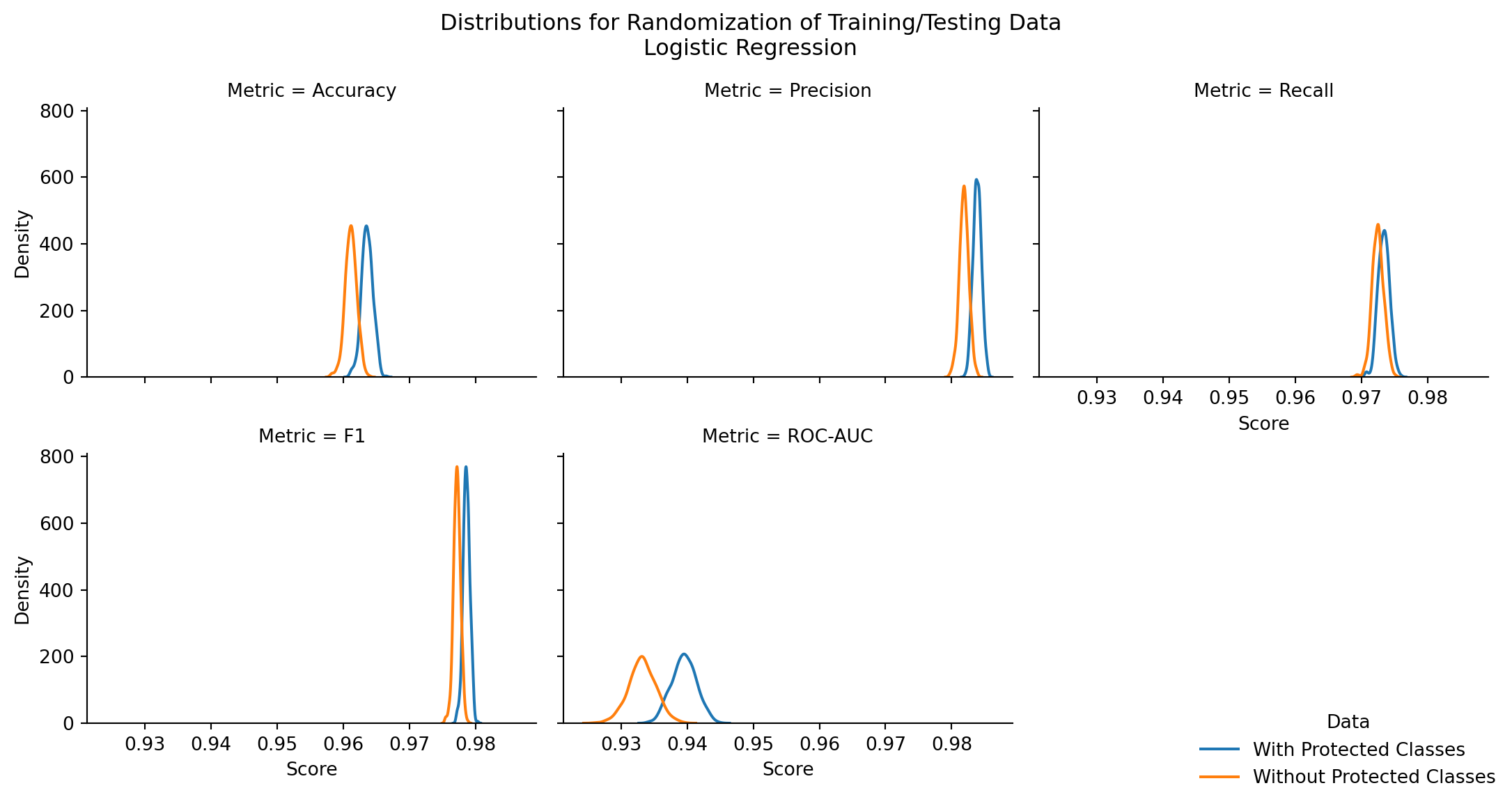
There is a chance that the difference in performance of the models trained with and without protected class data could be due to random chance, namely the random splitting of training and testing data from the source datasets.
To examine the potential for the difference (albeit minute) between both modeling methods, one can conduct a randomization test on the source data itself to examine for a statistically significant difference in means.
To do so, one can shuffle the data multiple times into new training and testing datasets, re-train the models, and capture the performance scores of each model (one trained with, and one trained without, protected classes). From here, one achieve’s a distribution of the performance scores (such as Accuracy, Precision, Recall, F1, and ROC-AUC scores) of each model; when the number of randomizations increase, the distribution of each should approach a normal distribution.
To perform the randomization, the data was shuffled 500 times, and two models were trained on each shuffle, capturing the aforementioned scores. When these shuffles were executed, the following outcomes were achieved:
Figure 9.2
Table 9.11: Per Metric Paired Z-test (Logistic Regression, 500 Iterations)
Stat
z-score
p-value
top performer
top mean
difference in means
Accuracy
44.648798
0.000000
With Protected Classes
0.963586
0.002457
Precision
47.173034
0.000000
With Protected Classes
0.983867
0.001985
Recall
16.219786
0.000000
With Protected Classes
0.973386
0.000889
F1
43.977874
0.000000
With Protected Classes
0.978598
0.001431
ROC-AUC
50.590439
0.000000
With Protected Classes
0.939526
0.006305
One can see that over 500 iterations of shuffling nearly 200k records, that the model trained on the multiple correspondence analysis that included protected class information had statistically better performance across all metrics.
This is a substantial finding. Namely, these significant difference signifies that including protected class information in logisitic regression confidently improves its predictive performance, better than if it were excluded as part of the model training data.
Furthermore, in comparison to all Naive Bayes models and all decision tree models, including their randomization testing, the Logistic Regression model outperforms them all in every metric. The most discerning factor is the fact that the ROC-AUC score for Logistic Regression is in the 90s, whereas few if any other ROC-AUCs for other models exceeded 89%.
What does this mean? It means that, if using logistic regression modeling to assess whether or not a loan should be approved, that a company could choose to include protected class data when building a linear regression model if they’re concerned about model performance.
Ethically speaking, however, it should be excluded outright. This is further evidenced by the overall difference in performance between two models trained on the exact same data, less protected class variable presence. The difference, while statistically significant, is not operationally significant, as the maximum difference in means for each performance metric is less than 0.6%.
Leveraging that ethical perspective, while the difference is significantly different, from a mathematical standpoint, that models leveraging protected class information outperform those that exclude it, the cost is minimal. Exclustion of protected class information still achieves incredibly high accuracy, precision, Recall, F1, and ROC-AUC, all ranging from 93%-98% to make predictions. Such modeling can be leveraged to inform one as to the likely outcome of the loan application, and can be leveraged in conjunction with other available relevant information to make an informed decision.
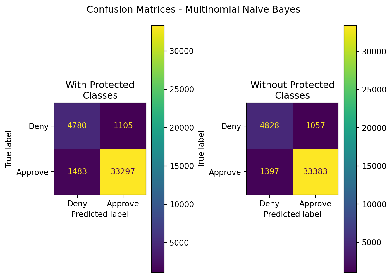
9.4.2 Multinomial Naive Bayes
The results here are the same as included and described within Chapter 7. The findings are the same.
Examining MultinomialNB’s performance, it seems to have fairly low performance in terms of accuracy. This is likely caused by the fact that it was provided with Bernoulli data, as it was the only way to obtain count data from the source records. That being said, the performance is quite precise.
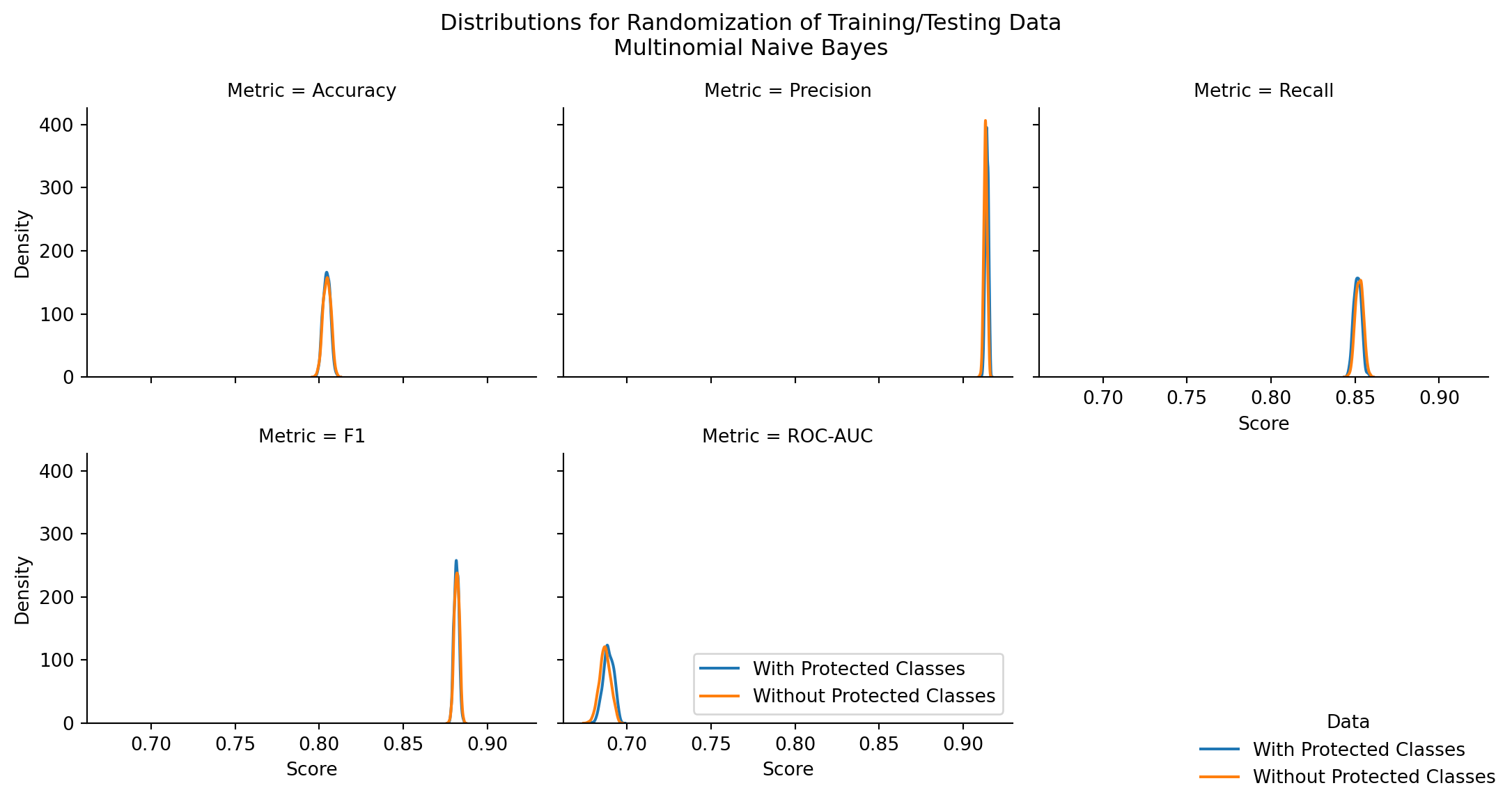
Across 500 iterations of MultinomialNB, there was not a significant difference in accuracy or F1 score of the models when they were and when they weren’t trained with protected class information. For other cases, the difference, while statistically significant, was within 1 percentage point of the top performer. Operationally speaking, there’s not a substantial need for that level of performance. The protected class information inclusion or exclusion makes a statistically significant, but not operationally impactful, difference in model performance.
9.5 Overall
The performance of Logistic Regression, with and without protected classes, far outshined the performance of Multinomial Naive Bayes. Multinomial Naive Bayes may have had better performance had the data provided the opportunity to better be count-vectorized, and as such is better suited for assessing document classification than individual record classification.
Another difference in the models is what they do and how they do it. Logisitic Regression is discriminative, meaning that we know the potential output classes and one crafts the model to maximize the likelihood of predicting a correct probability for a class, given new input data. MultinomialNB, however, is generative and seeks to identify the probability of the data, given a class.
Thus far, Logistic Regression’s accuracy (along with other metrics) makes it a top contender for modeling. This, however, comes at the cost of substantial dimensionality to explain approximately 99.99% of the variance in the data with the MCA execution. If dimensionality reduction, computational memory and time were a constraint, it may render the execution of future predictions with logisitic regression infeasible. This especially becomes the case when the model needs to be refit with additional new data; the sheer volume of features and row vectors produces a tremendous amount of data (near 1 Gb), and the execution of gradient descent upon said data to produce a well-performing logisitic regression is also computationally expensive and time consuming.