3  Principal Component Analysis

3.1 Overview

Principal component analysis (or PCA) is the act of rotating in combination with stretching or squishing the axes of a multi-dimensional dataset to better align with its direcitonality in multidimensional space. By realigning the axes, the variation within the data can be more directly tied to and explained by the axes (also called Principal Components). In some cases, the transformation can be so profound such that a substantial amount of the data’s variation can be explained using fewer dimensions.

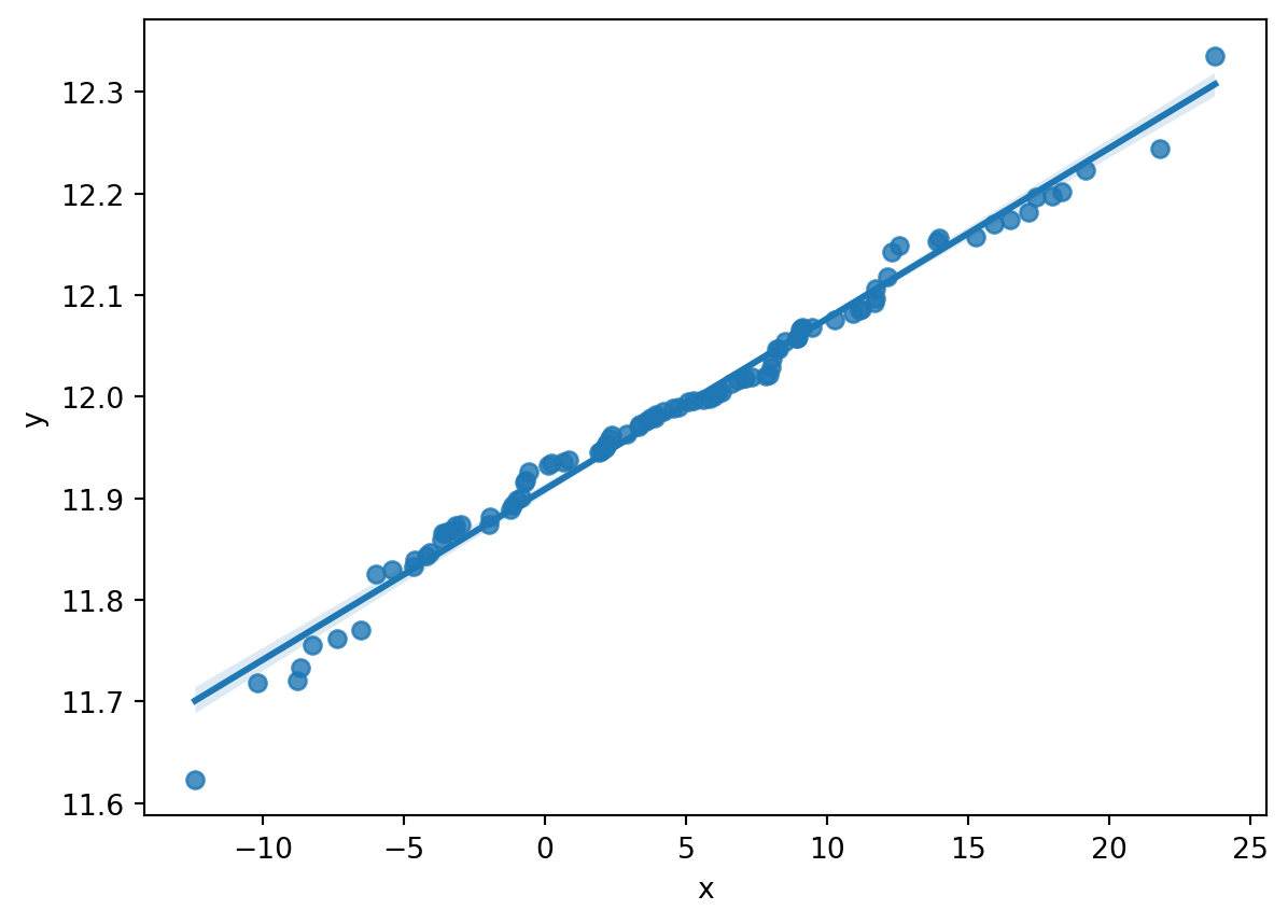
Consider the below graphic:

Figure 3.1: A strongly correlated 2-dimensional dataset

The X and Y values of this data appear to be connected, correlated even. Note - PCA is NOT a correlation analysis, but leverages any existing correlation in the data between one or more variables to transform the basis of each datapoint and vector in the data.

The goal of PCA is to remove strong corrlelations with high R values from the data by realigning axes of the data along the directions in the data which contain the greatest variance in the data. The above plot appears to show that the x-coordinate is a good predictor for the y-coordinate, and a simple linear regression analysis reveals that this is the case.

Table 3.1: Least Squares Regression, before PCA

OLS Regression Results

Dep. Variable:	y	R-squared:	0.985
Model:	OLS	Adj. R-squared:	0.985
Method:	Least Squares	F-statistic:	6400.
Date:	Tue, 10 Dec 2024	Prob (F-statistic):	4.49e-91
Time:	08:20:54	Log-Likelihood:	274.70
No. Observations:	100	AIC:	-545.4
Df Residuals:	98	BIC:	-540.2
Df Model:	1
Covariance Type:	nonrobust

	coef	std err	t	P>|t|	[0.025	0.975]
const	11.9091	0.002	6468.253	0.000	11.905	11.913
x1	0.0168	0.000	80.000	0.000	0.016	0.017

Omnibus:	41.522	Durbin-Watson:	0.564
Prob(Omnibus):	0.000	Jarque-Bera (JB):	139.401
Skew:	-1.374	Prob(JB):	5.36e-31
Kurtosis:	8.089	Cond. No.	10.4

Notes:
[1] Standard Errors assume that the covariance matrix of the errors is correctly specified.

Imagine instead if the axes, while retaining their perpendicularity (or orthogonality), streched in the general orientation of the regression line (we’ll call it \(X'\) or our new X axis) from Figure 3.1, with \(Y'\) bisecting \(X'\) at a \(90^o\) angle. Below is a depiction of the data after such a transformation.

Figure 3.2: the 2D dataset, post PCA transformation

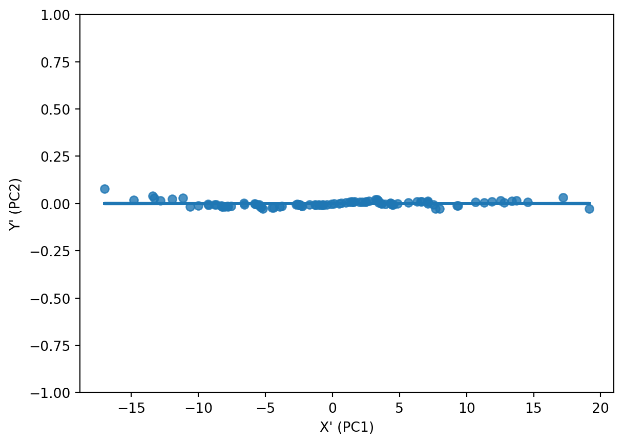
Figure 3.2 shows us that after the transformation, the data has a correlation value closer to zero than having a strong positive value as it had within Figure 3.1. One might also note that Y’ is an directional inversion of Y in this case (e.g. values that were above the correlation plot line in Figure 3.1 are below the correlation line in Figure 3.2). The act of applying PCA transformation is a linear combination that can result in the rotation, expansion and/or contraction of a vector as it is transposed into the new basis space.

Performing regression analysis on this data once more reveals that the goal of PCA is reached, that the variables, when projected into this new basis, hold no correlation:

Table 3.2: Least Squares Regression, after PCA

OLS Regression Results

Dep. Variable:	y	R-squared (uncentered):	0.000
Model:	OLS	Adj. R-squared (uncentered):	-0.010
Method:	Least Squares	F-statistic:	0.000
Date:	Tue, 10 Dec 2024	Prob (F-statistic):	1.00
Time:	08:20:54	Log-Likelihood:	274.71
No. Observations:	100	AIC:	-547.4
Df Residuals:	99	BIC:	-544.8
Df Model:	1
Covariance Type:	nonrobust

	coef	std err	t	P>|t|	[0.025	0.975]
x1	2.168e-19	0.000	1.04e-15	1.000	-0.000	0.000

Omnibus:	41.519	Durbin-Watson:	0.564
Prob(Omnibus):	0.000	Jarque-Bera (JB):	139.378
Skew:	1.374	Prob(JB):	5.43e-31
Kurtosis:	8.089	Cond. No.	1.00

Notes:
[1] R² is computed without centering (uncentered) since the model does not contain a constant.
[2] Standard Errors assume that the covariance matrix of the errors is correctly specified.

Considering the tightness of all of the datapoints in Figure 3.2 to the \(X'\) / PC1 axis, along with the total lack of correlation between the variables, one could potentially discard or disregard the \(Y'\) / PCA2 axis for the purpose of modeling.

Absent the PCA transformation, one could discard the y-datapoints and retain solely the x datapoints and the linear regression line equation \(y=mx+b\) between x and y such that one could re-calculate the y-value on-the-fly.

By performing PCA and transforming the variables in lieu of performing a recalculation of the y-value using the regression equation, the user can simply assume y to be zero in all cases and simply disregard the value. This allows the user to completely eliminate the feature while simultaneously retaining a high degree of explainability of variance within the data.

The eigenvalues of a PCA conveys the importance, and almost weight, of its corresponding eigenvector in explaining variation within the data. The eigenvalues are calucated from the covariance matrix of the original data, and then sorted in descending order, and then the corresponding eigenvectors, or basis vectors, are calculated and stored in a matrix. From here, eigenvalues and eigenvectors are pruned from the calculation based upon the needs of the user.

The dot product of the remaining eigenvectors and the original data then produce the PCA-transformed data.

The ratio of an individual eigenvalue over the sum total of all eigenvalues corresponds to an aforementioned weight or importance the corresponding eigenvector holds. This ratio corresponds to the amount of variance that is explained by the eigenvector and eigenvalue within the source data.

In best-case scenarios, one may have a high volume of dimensions, and many of those dimensions may have connections, correlations, or generally trend together. Due to the sheer volume thereof, it’s near impossible to visually inspect, determine, and prune correlated features from data. PCA, in the best case, allows a researcher to mathematically identify and trim all such correlations from the data, and capture all variation of the data within a fraction of the original dimensions.

3.2 PCA in this Study

This study will explore PCA of select quantitative features of the cleaned dataset. While this will be explored, it is not necessarily ideal for the purpose and intent of this study.

When leveraging principal components, one loses a degree of explainability for the data, and one arrives at a frame of reference that is not fully intuitive or easily digested. Each of the newly aligned axes, or principal components, is a linear combination of the original axes, and each datapoint is a combination of multiple features (e.g. the sum of 0.8 times feature A, 3.7 times feature B, 2.6 times feature C, as an arbitrary example). This makes the inputs and outputs less interpretable under direct observation.

This study is exploring the impact of categorical and numeric features and the strength of their predictive power in determining results or sources, i.e. 

• Can one better predict mortgage outcomes (e.g. interest rate, approval or denial) from HMDA data when protected classes are included as predictors?

• Can one predict ones protected classes when using other available data about properties of the loan and the property it would purchase?

• How strongly do these features lend themselves to such predictions?

With research questions like these in mind, performing PCA is less beneficial to explaining the outcomes.

If the HMDA data were to be used in conjunction with additional numerical information on the potential borrower, however, leveraging PCA could be of benefit. For instance, if additional features about the borrower such as total liquid savings, total invested dollars, credit score, age of credit history, and a substantial volume of other numeric variables, leveraging PCA could be beneficial in supporting assessment and analysis.

If a PCA of all of those numerics reduced the volume or dimension of the original data from, perhaps 20 to 5 features, it would simplify the process of training machine learning models. Whether building a multi-layer perceptron, performing a grid search with cross-validation of multiple model hyperparameters for models like logistic regression, support vector machines, ridge classifiers, or others - the reduction in dimensions reduces the computational time and complexity required to attain a more optimally-performing model.

3.3 Data

To perform PCA, there are a few requirements to ensure that the outcomes are relevant, valid, and (potentially) useful:

• The data must not contain any labels (e.g. the dependent or response variable)

• The data must include solely numeric data

  • The data must be standard scaled by the formula \(\frac{x-\mu}{\sigma}\) where \(x\) is the variable in question, \(\mu\) is the mean of \(x\), and \(\sigma\) is the standard deviation of \(x\)

    • Failure to perform this standard scaling will allow features with larger magnitudes to have a stronger impact on the outcome. To compare variances and the degree of explained variance, all features need to be on the same scale for comparison during PCA.

  • There are variables that may be represented as numbers in a source dataset, but the numbers leveraged in PCA must truly be numbers

  • Remapping of categorical data to numbers cannot be performed

• When reducing dimensions in the transformed data, seek to retain a high degree of cumulative explained variance with the minimum number of dimensions required to achieve it

With these things in mind, only a small subset of the columns from the cleaned and consolidated HMDA dataset meet the numeric requirement for PCA. These columns include:

Table 3.3: Numeric Columns Leveraged for PCA

variable
property_value
lender_credits
discount_points
origination_charges
total_loan_costs
property_value
income
total_units
tract_median_age_of_housing_units
tract_minority_population_percent
loan_to_value_ratio
debt_to_income_ratio

From the initial efforts in data collection, all of these columns hold numeric and non-null data points to support calculation.

The data used to perform PCA is located here.

Data before Standard Scaling is as follows:

Table 3.4: data, pre-standardization

income	interest_rate	total_loan_costs	loan_to_value_ratio	loan_term	intro_rate_period	total_units	tract_minority_population_percent	tract_population	tract_to_msa_income_percentage	tract_owner_occupied_units	tract_one_to_four_family_homes	tract_median_age_of_housing_units
95.500000	4.250000	18615.000000	85.000000	360.000000	120.000000	1	17.150000	5599	130.240000	2248	2492	36
0.000000	4.250000	5907.500000	21.429000	360.000000	120.000000	1	13.370000	3911	292.450000	1239	142	0
607.000000	5.250000	3055.000000	80.000000	360.000000	84.000000	1	35.670000	10542	292.450000	753	48	0
202.000000	5.125000	7322.120000	92.175000	360.000000	60.000000	1	40.330000	22780	276.610000	5430	6341	12
298.000000	5.625000	5325.000000	65.574000	360.000000	84.000000	1	19.470000	3344	193.660000	1061	1128	69

Table 3.5: data, ,post-standardization

	income	interest_rate	total_loan_costs	loan_to_value_ratio	loan_term	intro_rate_period	total_units	tract_minority_population_percent	tract_population	tract_to_msa_income_percentage	tract_owner_occupied_units	tract_one_to_four_family_homes	tract_median_age_of_housing_units
0	-0.094708	-3.227802	3.056869	0.264355	0.236292	6.982175	-0.099862	-0.921922	0.337094	0.390175	1.745898	1.286805	-0.028225
1	-0.292129	-3.227802	-0.054903	-2.930017	0.236292	6.982175	-0.099862	-1.068476	-0.463000	4.060474	0.030686	-2.060488	-1.928347
2	0.962682	-1.809658	-0.753414	0.013111	0.236292	4.823390	-0.099862	-0.203884	2.680023	4.060474	-0.795472	-2.194380	-1.928347
3	0.125452	-1.986926	0.291505	0.624891	0.236292	3.384200	-0.099862	-0.023212	8.480705	3.702065	7.155021	6.769243	-1.294973
4	0.323907	-1.277854	-0.197544	-0.711780	0.236292	4.823390	-0.099862	-0.831973	-0.731752	1.825169	-0.271899	-0.656050	1.713554
...	...	...	...	...	...	...	...	...	...	...	...	...	...
203316	0.168864	0.140289	0.429219	-0.489378	0.236292	-0.213775	-0.099862	0.392025	-0.670134	-1.093014	-1.274848	-0.883950	1.344085
203317	1.409205	0.140289	0.429219	-0.238134	0.236292	-0.213775	-0.099862	1.187992	-0.169601	-2.556744	-0.044111	-0.505065	-0.608818
203318	0.108914	-0.036979	0.265745	-0.991867	0.236292	-0.213775	-0.099862	0.177622	1.465188	0.695637	0.987737	0.783999	-1.400535
203319	-0.197036	0.140289	0.326358	0.867342	0.236292	-0.213775	-0.099862	-0.046862	-0.647382	-0.420318	-0.530286	-0.509338	0.552368
203320	-0.046128	0.140289	-0.032444	0.013111	0.236292	-0.213775	-0.099862	-1.367012	-0.509925	0.404430	0.251674	0.033350	0.446806

203321 rows × 13 columns

3.4 Code

The code used to perform PCA is located here.

3.5 Principal Component Analyses

3.5.1 2D PCA

Table 3.6: 2D PCA Calculation

PC	Eigenvalues	Cumulative Variance
PC1	2.772669	0.213281
PC2	1.477353	0.326923

The 2D PCA achieves an explanation of approximately 32.6% of the variance in the source data.

Figure 3.3: 2D PCA Visualization Plot

3.5.2 3D PCA

Table 3.7: 3D PCA Calculation

PC	Eigenvalues	Cumulative Variance
PC1	2.772669	0.213281
PC2	1.477353	0.326923
PC3	1.225321	0.421178

The 3D PCA achieves an explanation of approximately 42.1% of the variance in the source data.

Figure 3.4: 3D PCA Visualization

3.5.3 Multi-Dimensional PCA

Table 3.8: Eigenvalues and Variance, all dimensions

PC	Eigenvalues	Cumulative Variance
PC1	2.772669	0.213281
PC2	1.477353	0.326923
PC3	1.225321	0.421178
PC4	1.123168	0.507575
PC5	1.047675	0.588165
PC6	0.976401	0.663273
PC7	0.967920	0.737728
PC8	0.931685	0.809395
PC9	0.810819	0.871766
PC10	0.700385	0.925641
PC11	0.633995	0.974410
PC12	0.218066	0.991184
PC13	0.114606	1.000000

The top three eigenvalues / eigenvectors are highlighted in each of Table 3.6, Table 3.7, and Table 3.8, of 2.77, 1.477, and 1.225.

To retain a minimum of 95% of the information in the dataset, the minimum required principal components are 11, allowing for dimensionality reduction of 2 dimensions from the original 13 while retaining the required amount information. The lowest value greater than 0.95 in the cumulative variance column is on the 11th row for Principal Component 11 at 0.974, thus one would have to include all components 1-11 to achieve at least 95% explained variance.

This finding suggests that the source data do not have strong correlations with one another, and thus do not provide much assistance in reducing dimensionality.

3.6 Multiple Correspondence Analysis

Many of the research questions within this effort are inherently linked to categorical factors in lieu of numeric factors. Principal component analysis is only executable upon numeric data and not upon categorical data - even in the case of ordinal data. As a simple example, consider a ordinal variable “size” with categories small, medium, large, and extra-large. One could apply a simple encoding and assign small=1, medium=2, large=3, and extra-large=4. This encoding, while apparently holding a degree of validity in terms of increasing size, does not match up mathematically to reality. Consider getting a fountain drink at a fast-food restaurant and ask the question - is a large the same as 3 smalls? Is an extra large the same as 1 medium and two smalls? Rarely are either of these answers “yes”. One might have to add decimal places to the categories, and at that point, one may as well get the exact size measurements in terms of fluid ounces or liters, which may or may not be possible.

The additive and multiplicative challenges between these categories when assigning them a value produces challenges for ordinal variables. These challenges are further confounded when pivoting away from an ordinal variables. One runs the risk of making mathematical claims such as red is 4 times blue, or that sad is 3 less than happy. Such statements are nonsensical, have no foundation in mathematics, and while they may produce results in a model post-transformation, do not hold validity, explainability, or generalizability.

Enter Multiple Correspondence Analysis (or MCA). MCA performs an analogous action on categorical variables as PCA performs upon numeric variables. To perform an MCA, one must construct a Complete Disjunctive Table, which is effectively a one-hot encoded matrix. One takes the source categorical columns and transforms them to a column per category, and for the new column, the value is set to 1 if the current row is a member of the category, and zero otherwise. This is repeated for all columns and categories until the dataset is fully expanded.

a	b
s	f
m	w
s	s
s	f
m	f
m	f
l	w
l	s
l	f
m	w

Taking the above example table, one can transform it to a one-hot encoded table:

a_l	a_m	a_s	b_f	b_s	b_w
0	0	1	1	0	0
0	1	0	0	0	1
0	0	1	0	1	0
0	0	1	1	0	0
0	1	0	1	0	0
0	1	0	1	0	0
1	0	0	0	0	1
1	0	0	0	1	0
1	0	0	1	0	0
0	1	0	0	0	1

Notice that there are now have 6 columns from the original 2 columns. This is because column ‘a’ had 3 categories - s/m/l, as did column ‘b’ - s/w/f. A column is created for each combination of individual columns and their respective categories, hence 6 columns in this case.

After performing this transformation, the following mathematical operations are applied:

• Calculate the sum of all values (0s and 1s) from the CDT as value \(N\)

• Calculate matrix \(Z = \frac{CDT}{N}\)

• Calculate the column-wise sum as matrix \(c\). Transform to a diagonal matrix \(D_c\)

• Calculate the row-wise sum as matrix \(r\). Transform to a diagonal matrix \(D_r\)

• Calculate matrix \(M = D_r^{-\frac{1}{2}}(Z-rc^T)D_c^{-\frac{1}{2}}\)

Due to some unforeseen challenges during this research, performance of MCA will be delayed until a later date. This type of analysis will be useful for future modeling purposes and further analysis.

3.7 Results

Principal component analysis on the source data for this research is not an ideal endeavor, as this effort seeks to further establish the strength and connection of certain numeric and categorical variables to the outcome of whether or not an applicant will attain a mortgage.

Furthermore, the need of the data to retain 11 of the 13 principal components to explain most of the data variation means that applying PCA to this data will not meet any dimensionality reduction goals for this research. There is little direct correlation between the variables in the source data, so it takes almost the same number of dimensions as we had in the source data to retain a high degree of explainability. As such, principal component analysis, solely performed on the identified numeric variables, may be insufficient for the purposes of clustering and modeling.

The multiple correspondence analysis, however, seems to lend itself well to the purposes and intent of this research. A limited degree of exploration into MCA was pursued, but not sufficiently enough to generate or communicate results at this time. In the next iteration of this research, MCA will be included in the analyses. MCA, used within clustering and potentially within modeling, could be more relevatory than basic numeric measures provided by PCA.