Decision trees, when constructed and visualized are one of the machine learning models that are most easily understood by humans on direct examination. A decision tree provides a root node, multiple decision nodes, and branches to follow based upon the current decision node. Each node provides some sort of decision based upon a feature or variable for an input record.
The decision tree is, then, quite akin to a flowchart. Employers around the globe use flowcharts to explain processes and procedures to their employees to simplify workflows and provide a frame of reference to get things done. As such, decision tree machine learning modeling is user-friendly, easily-understood, and readily consumed. Decision trees are be high-utitlity, both to human users as well as well as for computers with their very simple branching logic.
8.1.1 How Does One Build a Decision Tree?
The process of building a decision tree has some math behind it, but is fairly simple to explain without the math. To proceed in processing, one needs data in the appropriate format (in Python, the requirement is numeric data only, using available packages). Once the data is in hand, it must be split into a training and testing dataset. From here, we can use the following step(s) to proceed building the tree.
Select a heuristic that will measure the how impure the current state of the data is, at the current node.
Select a maximum depth to which your tree will grow, so as to prevent over-fitting. Too small a value can result in under-fitting (poor model performance)
While we haven’t reached the maximum depth:
for each feature in the current partition of the dataset (starting with the full dataset):
calculate the heuristic for each value of the current feature if it were to be split on the value
using the heuristic, calculate the information gain if the data were to be split on the feature
for the feature value with the highest information gain, split the data on the feature’s value for instance, if the feature were “cost”, the condition could be “cost <= 100?”, and divide the data into two pieces, one where the condtion is true, the and the other where it is false. Increment the depth of our tree.
repeat process for the two new partitions if the heuristic is greater than zero
if it is zero, then the partition is considered pure. This signifies that all records in the partition are members of the same class, and this node can be used to clearly make a decision of the class of a future input object.
This is all fine and good in terms of understanding steps to produce the tree - but what are heuristics and information gain? How can one calculate them and leverage them to execute this process?
8.1.2 Heuristics
Common heuristics for measuring the current state of a data partition include Gini indexing and Entropy measures. These values give a sense of how impure the current state of the data is. These heuristics support the splitting of the data at nodes in the tree to reduce the impurity.
For calculating gini, one iterates over the current split of the data and calculates the sum total members in each class for the current node out of the total number of records in the current node, squares them, and takes the sum total thereof, and subtracts it from one.
Gini being 0 signifies that the node is pure and the algorithm can stop executing on this branch. Mathematically speaking, this is only possible when the records in the current node all belong to one class (e.g. pure). One seeks with each split to reduce the Gini index by the maximum value possible with each node split.
Entropy takes the same calculation as done in gini - the number of records in the current data split of a specific class out of the total number of records in the split. What entropy does differently is that it multiplies that value by it’s base 2 logarithm, sums the total values, and takes the negative (which must be done as logarithms with fractional inputs produce negative numbers). Calculating by hand gets hairy if you’re not paying attention. Technically speaking, a logarithm with an input of 0 is undefined. However, when the input to the log is zero, so is its external multiplier. The external multiplier is used as the discriminating factor and the result is set to zero.
Entropy being 0 signifies that the node is pure and the algorithm can stop executing on this branch. One seeks with each split to reduce the entropy by the maximum value possible with each node split.
For both metrics, the best case scenario is a pure node with heuristic = 0. The worst case, mathematically, is 0.5 for Gini and 1 for Entropy.
8.1.3 Information Gain
The following equation outlines the calculation for information gain at each split of a decision tree:
\(h_{i-1}\) is the heuristic (Gini or Entropy) of the previous node (i.e. impurity). \(h_i\) is the current proposed split, \(N\) is the number of available splits to perform with the current data, \(D_j\) is a proposed split of the data for building a new node on column \(j\in N\), and \(G_i\) is the information gain for the current proposed split.
The algorithm selects the highest \(G_i\) as the winner for where and how to split the current state of the data, and repeats to a certain specified depth, or until the algorithm has pure nodes as leaves.
8.1.4 Summary of Metrics
Using a heuristic like gini or entropy provides a measure of pureness for the current state of the dataset. When leveraging information gain, it tells one how much a proposed split would reduce the impurity in the data (or conversly, how much additional information one would have available in the data if one were to split on the current feature value). By choosing the maximum value for information gain we are selecting the option which most greatly reduces the impurities present in the data.
8.1.5What challenges exist with decision trees?
There are several considerations when building a decision tree. The intent as discussed in the overview of this section is to provide an easily understood and accessible model that delivers reasonably good peformance. As such, a decision tree should be readable and not overwhelming. To meet this need, the tuning of the tree’s maximum depth is necessary so as to ensure the resulting tree is reasonably sized and can be followed by its users.
Similarly, tree depth also assists one in overcoming a decision tree’s challenges with over and underfitting. Higher depth will improve the accuracy of future predictions by the tree, but at the cost of readability. Having too high of a depth is problematic as well. Since the algorithm seeks to have all leaf nodes at the base of the tree be as pure as possible, an unconstrained algorithm will continue splitting the data until this condition is met. This can result in leaves on the tree containing single node outcomes, which is an overfitting condition. Having too small of a depth can provide a simple tree, but at the cost of performative accuracy.
Decision trees can be fast, however, building the tree when using a large volume of training data can be computationally expensive.
Trees can also have challenges with performing updates. The trees are pre-trained, and as new records are added to training data, the addition thereof changes the hueristic value from what it was previously for each variable value under consideration. As such, the tree would need to be reconstructed when new data is made available for training.
Decision trees also, in nearly every case, can have infinitely many possible tree outcomes. Specifically, any dataset that contains numeric data (continuous), the possibilities are endless.
8.2 Data and Code
Multiple data formats were leveraged to produced multiple decision trees, with and without protected class information.
One version of the tree production leveraged the multiple correspondence analysis outputs produced within Appendix G, with and without protected class information.
Another version of tree production leveraged label encoded data that was previously produced in Appendix D. Since label-encoded data was necessary to perform Categorical Naive Bayes, this same data, as a numeric, has utility for decision tree building.
Summarized views for the training and testing data are in the below tables:
Table 8.1: Decision Tree Training Data (With Protected Class)
derived_sex
preapproval
open-end_line_of_credit
loan_amount
loan_to_value_ratio
interest_rate
total_loan_costs
origination_charges
discount_points
lender_credits
...
co-applicant_ethnicity_No Co-applicant
aus_Desktop Underwriter
aus_Loan Prospector/Product Advisor
aus_TOTAL Scorecard
aus_GUS
aus_Other
aus_Internal Proprietary
aus_Not applicable
aus_Exempt
outcome
142289
3
0
1
1
2
3
1
1
1
1
...
0
1
0
0
0
0
0
0
0
1.0
174168
0
0
1
2
2
3
1
1
1
1
...
1
1
0
0
0
0
0
0
0
1.0
106229
1
1
1
1
2
2
1
1
1
1
...
0
1
0
0
0
0
0
0
0
0.0
30766
0
1
1
3
2
2
3
1
1
1
...
1
1
1
0
0
1
0
0
0
1.0
34556
0
1
1
1
2
2
1
1
1
1
...
1
1
1
0
0
1
0
0
0
1.0
60130
0
1
0
1
1
2
1
1
1
1
...
1
0
0
0
0
0
0
1
0
0.0
114480
0
0
1
1
4
2
1
1
1
1
...
1
1
0
0
0
0
0
0
0
1.0
61174
2
1
1
1
2
2
1
1
1
1
...
1
0
1
0
0
0
1
0
0
0.0
131619
2
0
1
1
4
2
1
1
1
1
...
0
1
0
0
0
0
0
0
0
1.0
77029
2
1
1
2
2
2
1
1
1
1
...
1
1
1
0
0
0
1
0
0
0.0
10 rows × 101 columns
Table 8.2: Decision Tree Testing Data (With Protected Class)
derived_sex
preapproval
open-end_line_of_credit
loan_amount
loan_to_value_ratio
interest_rate
total_loan_costs
origination_charges
discount_points
lender_credits
...
co-applicant_ethnicity_No Co-applicant
aus_Desktop Underwriter
aus_Loan Prospector/Product Advisor
aus_TOTAL Scorecard
aus_GUS
aus_Other
aus_Internal Proprietary
aus_Not applicable
aus_Exempt
outcome
89944
1
1
1
1
2
2
1
1
1
1
...
0
1
0
0
0
0
0
0
0
1.0
71083
1
1
1
1
1
4
1
1
1
1
...
0
1
0
0
0
0
0
0
0
1.0
44430
1
0
1
2
2
2
1
1
1
2
...
0
0
0
0
0
0
1
0
0
1.0
33808
2
1
1
1
2
1
0
0
1
0
...
0
0
0
0
0
0
0
1
0
1.0
101468
1
1
1
1
3
2
1
1
1
1
...
0
1
0
0
0
0
0
0
0
1.0
96435
2
1
1
1
2
2
1
1
1
1
...
1
1
0
0
0
0
0
0
0
1.0
64375
2
1
1
3
2
2
3
1
1
1
...
1
0
1
0
0
0
1
0
0
1.0
107749
0
1
1
1
2
2
1
1
1
1
...
1
1
0
0
0
0
0
0
0
1.0
40569
3
1
1
1
2
2
1
1
1
1
...
1
0
0
0
0
0
0
1
0
0.0
149685
3
1
1
1
2
2
2
2
2
1
...
1
0
1
0
0
0
0
0
0
1.0
10 rows × 101 columns
Table 8.3: Decision Tree Training Data (Without Protected Class)
preapproval
open-end_line_of_credit
loan_amount
loan_to_value_ratio
interest_rate
total_loan_costs
origination_charges
discount_points
lender_credits
loan_term
...
company
aus_Desktop Underwriter
aus_Loan Prospector/Product Advisor
aus_TOTAL Scorecard
aus_GUS
aus_Other
aus_Internal Proprietary
aus_Not applicable
aus_Exempt
outcome
142289
0
1
1
2
3
1
1
1
1
2
...
3
1
0
0
0
0
0
0
0
1.0
174168
0
1
2
2
3
1
1
1
1
2
...
3
1
0
0
0
0
0
0
0
1.0
106229
1
1
1
2
2
1
1
1
1
2
...
2
1
0
0
0
0
0
0
0
0.0
30766
1
1
3
2
2
3
1
1
1
2
...
1
1
1
0
0
1
0
0
0
1.0
34556
1
1
1
2
2
1
1
1
1
2
...
1
1
1
0
0
1
0
0
0
1.0
60130
1
0
1
1
2
1
1
1
1
2
...
0
0
0
0
0
0
0
1
0
0.0
114480
0
1
1
4
2
1
1
1
1
1
...
3
1
0
0
0
0
0
0
0
1.0
61174
1
1
1
2
2
1
1
1
1
2
...
0
0
1
0
0
0
1
0
0
0.0
131619
0
1
1
4
2
1
1
1
1
1
...
3
1
0
0
0
0
0
0
0
1.0
77029
1
1
2
2
2
1
1
1
1
2
...
4
1
1
0
0
0
1
0
0
0.0
10 rows × 34 columns
Table 8.4: Decision Tree Testing Data (Without Protected Class)
preapproval
open-end_line_of_credit
loan_amount
loan_to_value_ratio
interest_rate
total_loan_costs
origination_charges
discount_points
lender_credits
loan_term
...
company
aus_Desktop Underwriter
aus_Loan Prospector/Product Advisor
aus_TOTAL Scorecard
aus_GUS
aus_Other
aus_Internal Proprietary
aus_Not applicable
aus_Exempt
outcome
89944
1
1
1
2
2
1
1
1
1
2
...
4
1
0
0
0
0
0
0
0
1.0
71083
1
1
1
1
4
1
1
1
1
1
...
4
1
0
0
0
0
0
0
0
1.0
44430
0
1
2
2
2
1
1
1
2
2
...
0
0
0
0
0
0
1
0
0
1.0
33808
1
1
1
2
1
0
0
1
0
2
...
1
0
0
0
0
0
0
1
0
1.0
101468
1
1
1
3
2
1
1
1
1
2
...
2
1
0
0
0
0
0
0
0
1.0
96435
1
1
1
2
2
1
1
1
1
2
...
2
1
0
0
0
0
0
0
0
1.0
64375
1
1
3
2
2
3
1
1
1
2
...
0
0
1
0
0
0
1
0
0
1.0
107749
1
1
1
2
2
1
1
1
1
2
...
3
1
0
0
0
0
0
0
0
1.0
40569
1
1
1
2
2
1
1
1
1
1
...
1
0
0
0
0
0
0
1
0
0.0
149685
1
1
1
2
2
2
2
2
1
2
...
3
0
1
0
0
0
0
0
0
1.0
10 rows × 34 columns
As done in Chapter 7 for train test splits - the indexes are disjoint between training and testing datasets for each parent dataset (with and without protected classes), and each model is trained with the same records for comparison and evaluation against one another (same records for training and testing allow for direct comparison of the models).
By achieving these splits, the two models evaluated with and without protected class information will avoid unnecessary biases in the results. When a model is tested on data with which it has already been trained, the model has already optimized to the best of its ability to correctly classify the training data. As such, the outcome of an evaluation of a model using the same data in training and testing will artificially inflate its performance metrics (accuracy, precision, recall, F1, ROC-AUC). As such, it is paramount to have a disjoint training and testing dataset.
8.3 Results
Figure 8.1: Decision Tree (With Protected Classes)
Figure 8.2: Decision Tree (Without Protected Classes)
Table 8.5: Model Performance Scores (Single Run; D=4)
Model
Data
Accuracy
Precision
Recall
F1
ROC-AUC
Decision Tree
With Protected Classes
0.909013
0.911677
0.989477
0.948985
0.711476
Decision Tree
Without Protected Classes
0.909013
0.911677
0.989477
0.948985
0.711476
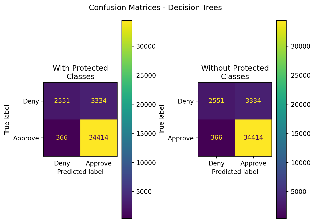
Figure 8.3: Decision Tree Confusion Matrices (With Protected Class Information; D=4)
By far and large, the most interesting result from this research are the decision trees produced for the data with and without protected classes
One can clearly see that the initially crafted trees are identical. While the numbers in terms of the value of each variable may not be clear (as they are a re-mapping of the source data from categories to integers), the gini index of each variable, and the variable names leveraged in decision making for building each tree, are incredibly clear.
The decision tree models for both datasets came to a concensus on how loan decisions could / should be made based upon highly relevant variables. Factors such as debt to income ratio, the loan’s proposed interest rate, the loan term, the automated underwriting system type, income, and whether or not the loan’s purpose was for an open end line of credit were the factors that most greatly partitioned each dataset so as to minimize the Gini index.
Many of the leaf nodes (where the decisions are made for classification) had remarkably low values for Gini index, within a tree depth of 6. The worst amongst these was with regard to the leaf nodes connected to automated underwriting systems, with Gini nearing the worst case scenario of 0.5. Separate of those, the decision trees were able to, fairly substantially, reduce the index closer to zero. An additional 1 or two layers to these trees may improve upon the result, but could also potentially render a decision-making process for loan approval or denial more complex.
Regardless, the result is astounding - for machine learning using decision trees, there is absolutely no impact to performance of the models when protected classes are included or excluded. These features do not provide sufficient enough information gain over other options to partition the dataset in a for the purpose of classification.
Furthermore - the performance of the decision tree is reasonably accurate as well, at or above 90%. If using ROC-AUC as a discriminating factor, however, this model could certainly benefit from additional tuning and adaptations. That being said, the other scores - depending on metric importance for decision making, all exceed the 90% watermark and are fairly good in terms of performance.
What if we prune some of the higher echelon features within the tree? What changes then?
First - let’s look at the tree by removing the root node. One can do this by removing the feature from the dataset and reconstructing the tree with the pruned data. In this case, that feature will be the debt to income ratio on the application.
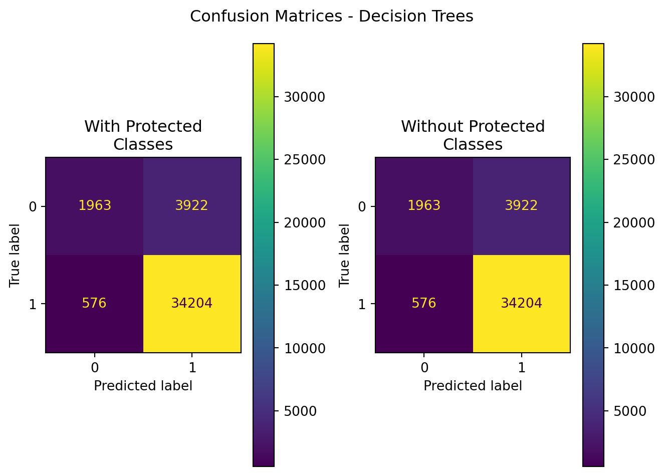
Figure 8.4: Decision Tree (With Protected Class Information; Feature Removed; D=4)
Figure 8.5: Decision Tree (Without Protected Class Information; Feature Removed; D=4)
Table 8.6: Model Performance Scores (Single Run; Features Removed; D=4)
Model
Data
Accuracy
Precision
Recall
F1
ROC-AUC
0
Decision Tree
With Protected Classes
0.889389
0.897131
0.983439
0.938304
0.658499
1
Decision Tree
Without Protected Classes
0.889389
0.897131
0.983439
0.938304
0.658499
Figure 8.6: Decision Tree Confusion Matrices (With Protected Class Information; Feature Removed; D=4)
We can see that after removing the debt_to_income_ratio feature from the data, that the decision tree with protected classes to begin including race and ethnic information as part of the decision making process. This includes Filipino co-applicants, and when co-applicant ethnicity is not provided on the application.
Despite that fact, however, the predicted outcomes (metric scores) are equivalent for each model.
Does this change any further when dropping automated underwriting systems from the training datasets (e.g. the root node of these new trees)?
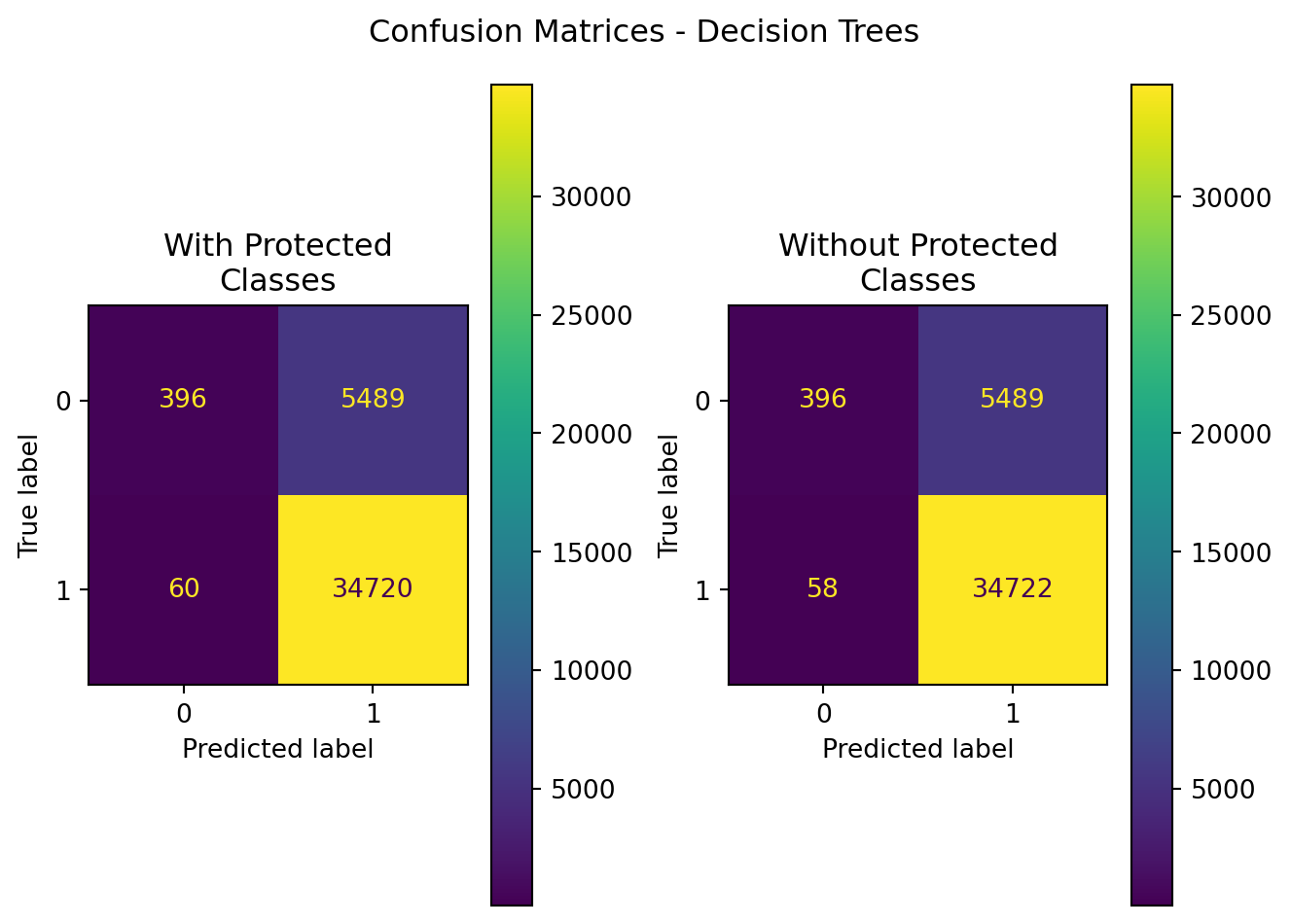
Figure 8.7: Decision Tree (With Protected Class Information; Features Removed; D=4)
Figure 8.8: Decision Tree (Without Protected Class Information; Features Removed; D=4)
Table 8.7: Model Performance Scores (Single Run; Features Removed; D=4)
Model
Data
Accuracy
Precision
Recall
F1
ROC-AUC
0
Decision Tree
With Protected Classes
0.863544
0.863488
0.998275
0.926002
0.532782
1
Decision Tree
Without Protected Classes
0.863593
0.863495
0.998332
0.926031
0.532811
Figure 8.9: Decision Tree Confusion Matrices (With Protected Class Information; Features Removed; D=4)
Here, we can see that the decision tree including protected class information picked up another deciding factor for race, substituting for the non-provided ethnic information. In this case, it has selected applicant race information unavailable as a splitting point in the tree. Examining the model performance metrics, we see that the decision tree without protected classes has improved performance over that of the tree that includes them.
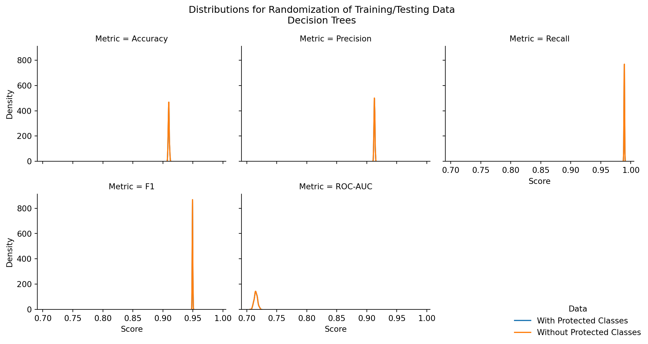
These trees were built off of a single iteration of training and testing splits. How do the performances of the two tree types (with and without protected class information) compare when performing the hypothesis testing outlined in Chapter 7.
Stat
z-score
p-value
top performer
top mean
difference in means
Accuracy
-0.063229
0.949584
Without Protected Classes
0.909842
0.000004
Precision
-0.048038
0.961686
Without Protected Classes
0.912724
0.000002
Recall
-0.045748
0.963511
Without Protected Classes
0.989174
0.000001
F1
-0.064089
0.948899
Without Protected Classes
0.949412
0.000002
ROC-AUC
-0.049822
0.960264
Without Protected Classes
0.715086
0.000009
Over 500 randomizations, there isn’t sufficient evidence to reject \(H_0\) - there is no significant difference between the two models. Surprisingly, the higher mean amongst all these insignificant test results had an insignificantly higher mean for each metric when protected class information was excluded. The p-values are incredibly high in these models, signifying a near total overlap in the mean and the variance of the data for both models’ performance metrics.
It appears the initial finding of the first two trees trained on the full dataset is clear: it is ideal to exclude protected class information of any kind when constructing decision tree models for mortgage application predictions. The accuracy of the decision tree without hyperparameter tuning is not a strong as what was found for Bernoulli Naive Bayes.