Appendix G — Multiple Correspondence Analysis

First, import the necessary modules

import pandas as pd, numpy as np, seaborn as sns, matplotlib.pyplot as plt

from sklearn.preprocessing import StandardScaler

from sklearn.decomposition import PCA

from sklearn.cluster import KMeans

from mpl_toolkits.mplot3d import Axes3D

from sklearn.preprocessing import OneHotEncoder

from prince import MCA

fr = pd.read_csv('../data/final_clean_r2.csv')

labels = fr['outcome'].copy()

G.1 Data Transformations

First, to perform MCA, variables require separation, and transformation to categorical variables. Below, the binary encoded fields for applicant race, ethnicity, and underwriting system, are broken back out into corresponding binary True/False columns for each category.

G.1.1 Breakout Race, Ethnicity, and Underwriting System Columns

##for use in splitting the collapsed columns 
##back out into their respective binary values
mapper = {
    'applicant_race':{
        'American Indian/Alaska Native':0b0000000000000000001,
        'Asian':0b0000000000000000010,
        'Asian Indian':0b0000000000000000100,
        'Chinese':0b0000000000000001000,
        'Filipino':0b0000000000000010000,
        'Japanese':0b0000000000000100000,
        'Korean':0b0000000000001000000,
        'Vietnamese':0b0000000000010000000,
        'Other Asian':0b0000000000100000000,
        'Black/African American':0b0000000001000000000,
        'Native Hawaiian/Pacific Islander':0b0000000010000000000,
        'Native Hawaiian':0b0000000100000000000,
        'Guamanian/Chamorro':0b0000001000000000000,
        'Samoan':0b0000010000000000000,
        'Other Pacific Islander':0b0000100000000000000,
        'White':0b0001000000000000000,
        'Information not provided':0b0010000000000000000,
        'Not Applicable':0b0100000000000000000,
        'No Co-applicant':0b1000000000000000000
    },
    'co-applicant_race':{
        'American Indian/Alaska Native':0b0000000000000000001,
        'Asian':0b0000000000000000010,
        'Asian Indian':0b0000000000000000100,
        'Chinese':0b0000000000000001000,
        'Filipino':0b0000000000000010000,
        'Japanese':0b0000000000000100000,
        'Korean':0b0000000000001000000,
        'Vietnamese':0b0000000000010000000,
        'Other Asian':0b0000000000100000000,
        'Black/African American':0b0000000001000000000,
        'Native Hawaiian/Pacific Islander':0b0000000010000000000,
        'Native Hawaiian':0b0000000100000000000,
        'Guamanian/Chamorro':0b0000001000000000000,
        'Samoan':0b0000010000000000000,
        'Other Pacific Islander':0b0000100000000000000,
        'White':0b0001000000000000000,
        'Information not provided':0b0010000000000000000,
        'Not Applicable':0b0100000000000000000,
        'No Co-applicant':0b1000000000000000000
    },
    'applicant_ethnicity':{
        'Hispanic/Latino':0b000000001,
        'Mexican':0b000000010,
        'Puerto Rican':0b000000100,
        'Cuban':0b000001000,
        'Other Hispanic/Latino':0b000010000,
        'Not Hispanic/Latino':0b000100000,
        'Information Not Provided':0b001000000,
        'Not Applicable':0b010000000,
        'No Co-applicant':0b100000000
    },
    'co-applicant_ethnicity':{
        'Hispanic/Latino':0b000000001,
        'Mexican':0b000000010,
        'Puerto Rican':0b000000100,
        'Cuban':0b000001000,
        'Other Hispanic/Latino':0b000010000,
        'Not Hispanic/Latino':0b000100000,
        'Information Not Provided':0b001000000,
        'Not Applicable':0b010000000,
        'No Co-applicant':0b100000000
    },
    'aus':{
        'Desktop Underwriter':0b00000001,
        'Loan Prospector/Product Advisor':0b00000010,
        'TOTAL Scorecard':0b00000100,
        'GUS':0b00001000,
        'Other':0b00010000,
        'Internal Proprietary':0b00100000,
        'Not applicable':0b01000000,
        'Exempt':0b10000000,
    }, 
}

new_mapper = {}
for k,v in mapper.items():
    new_mapper[k] = {}
    #print(k)
    for j,w in v.items():
        #print(w,j)
        new_mapper[k][w] = j

Next, the numeric variables require transformation to categorical. In this case, the standard deviation was leveraged to produce the following categories:

• Value < Mean - 2*standard deviation => L (low)

• Mean - 2 * standard deviation < Value < Mean - standard deviation => ML (Mid-Low)

• Mean - standard deviation < Value < Mean + standard deviation => M

• Mean + standard deviation < Value < Mean + 2 * standard deviation => MH (Mid-High)

• Value > Mean + 2 * standard deviation => H (High)

This categorization allowed for diversity in the source data prior to transforming with MCA

#adjust numerics to categoricals

#drop columns that will not be leveraged in MCA
fr.drop(
    labels = [
        'balloon_payment', 
        'interest_only_payment', 
        'other_nonamortizing_features',
        'income_from_median',
        'state_code',
        'county_code'
    ],
    axis=1,inplace=True
)

#identify numeric columns to convert to categorical
numerics = [
    'income',
    'loan_amount',
    'interest_rate',
    'total_loan_costs',
    'origination_charges',
    'discount_points',
    'lender_credits',
    'loan_term',
    'intro_rate_period',
    'property_value',
    'total_units',
    'tract_population',
    'tract_minority_population_percent',
    'ffiec_msa_md_median_family_income',
    'tract_to_msa_income_percentage',
    'tract_owner_occupied_units',
    'tract_one_to_four_family_homes',
    'tract_median_age_of_housing_units',
    'loan_to_value_ratio'
]

#set the cutting boundaries
bounds = [i/5 for i in range(1,5)]

for col in numerics:
    #income had some errors, for some reason
    if col == 'income':
        fr.loc[fr[col]<=0,col] = 0.01
        fr[col] = np.log(fr[col])

    s = fr[col].std()

    m = fr[col].mean()

    #cut everything based on standard deviations
    cut_level = [
        m-2*s,
        m-s,
        m+s,
        m+2*s
    ]
    
    cut_level = [-np.inf] + cut_level + [np.inf]

    #assign value based on cut boundaries
    fr[col] = pd.cut(
        fr[col],
        bins=cut_level,
        labels=["L","ML","M","MH","H"]
    )

    #convert to categorical
    fr[col] = fr[col].astype('category')

fr[numerics].head(10)

	income	loan_amount	interest_rate	total_loan_costs	origination_charges	discount_points	lender_credits	loan_term	intro_rate_period	property_value	total_units	tract_population	tract_minority_population_percent	ffiec_msa_md_median_family_income	tract_to_msa_income_percentage	tract_owner_occupied_units	tract_one_to_four_family_homes	tract_median_age_of_housing_units	loan_to_value_ratio
0	M	MH	L	H	H	M	H	M	H	M	M	M	M	M	M	MH	MH	M	M
1	L	MH	L	M	M	M	M	M	H	H	M	M	ML	M	H	M	L	ML	L
2	MH	H	ML	M	M	M	M	M	H	H	M	H	M	M	H	M	L	ML	M
3	M	MH	ML	M	M	M	M	M	H	M	M	H	M	M	H	H	H	ML	M
4	M	H	ML	M	M	M	M	M	H	H	M	M	M	H	MH	M	M	MH	M
5	MH	MH	M	MH	M	M	M	M	M	MH	M	M	ML	M	M	M	M	M	M
6	MH	H	M	M	M	M	M	M	MH	H	M	M	MH	M	M	M	M	M	M
7	MH	M	ML	M	M	M	M	M	M	H	M	M	ML	M	H	MH	ML	MH	L
8	M	H	ML	M	M	M	M	M	H	H	M	H	M	M	MH	MH	ML	H	M
9	M	M	ML	M	M	M	M	M	H	M	M	M	ML	M	MH	MH	M	ML	ML

After transforming numerics, the one-hot encoded columns extracted from race, ethnicity, and underwriting system required separation from the rest of the data so that all remaining categorical columns could be converted to a one-hot encoding.

Below outlines the separation of the race, ethnicity, and underwriting columns.

#extract binary columns
## because they're already one-hot encoded
fr_bin = fr[[
    'applicant_race',
    'applicant_ethnicity',
    'co-applicant_race',
    'co-applicant_ethnicity',
    'aus'
]].copy()

for k,v in new_mapper.items():
    for l,w in v.items():
        fr_bin[k+'_'+w] = (fr_bin[k]&l > 0).astype(int)

fr_bin.drop(
    labels=[    
        'applicant_race',
        'applicant_ethnicity',
        'co-applicant_race',
        'co-applicant_ethnicity',
        'aus'
    ],
    inplace=True,
    axis=1
)

fr.drop(
    labels=[
        'applicant_race',
        'applicant_ethnicity',
        'co-applicant_race',
        'co-applicant_ethnicity',
        'denial_reason',
        'aus', #may need to exclude this/comment it out...
        'outcome',
        'action_taken'
    ],
    inplace=True,
    axis=1
)
display(
    fr.head(10),
    fr_bin.head(10)
)

	derived_sex	purchaser_type	preapproval	open-end_line_of_credit	loan_amount	loan_to_value_ratio	interest_rate	total_loan_costs	origination_charges	discount_points	...	applicant_age	co-applicant_age	tract_population	tract_minority_population_percent	ffiec_msa_md_median_family_income	tract_to_msa_income_percentage	tract_owner_occupied_units	tract_one_to_four_family_homes	tract_median_age_of_housing_units	company
0	Sex Not Available	0	2	2	MH	M	L	H	H	M	...	3.0	7.0	M	M	M	M	MH	MH	M	JP Morgan
1	Male	0	2	2	MH	L	L	M	M	M	...	1.0	8.0	M	ML	M	H	M	L	ML	JP Morgan
2	Sex Not Available	0	1	2	H	M	ML	M	M	M	...	3.0	8.0	H	M	M	H	M	L	ML	JP Morgan
3	Male	0	2	2	MH	M	ML	M	M	M	...	4.0	8.0	H	M	M	H	H	H	ML	JP Morgan
4	Joint	0	2	2	H	M	ML	M	M	M	...	1.0	1.0	M	M	H	MH	M	M	MH	JP Morgan
5	Joint	0	1	2	MH	M	M	MH	M	M	...	2.0	3.0	M	ML	M	M	M	M	M	JP Morgan
6	Joint	0	2	2	H	M	M	M	M	M	...	2.0	1.0	M	MH	M	M	M	M	M	JP Morgan
7	Sex Not Available	0	1	2	M	L	ML	M	M	M	...	1.0	1.0	M	ML	M	H	MH	ML	MH	JP Morgan
8	Joint	0	1	2	H	M	ML	M	M	M	...	1.0	1.0	H	M	M	MH	MH	ML	H	JP Morgan
9	Sex Not Available	0	1	2	M	ML	ML	M	M	M	...	1.0	1.0	M	ML	M	MH	MH	M	ML	JP Morgan

10 rows × 37 columns

	applicant_race_American Indian/Alaska Native	applicant_race_Asian	applicant_race_Asian Indian	applicant_race_Chinese	applicant_race_Filipino	applicant_race_Japanese	applicant_race_Korean	applicant_race_Vietnamese	applicant_race_Other Asian	applicant_race_Black/African American	...	co-applicant_ethnicity_Not Applicable	co-applicant_ethnicity_No Co-applicant	aus_Desktop Underwriter	aus_Loan Prospector/Product Advisor	aus_TOTAL Scorecard	aus_GUS	aus_Other	aus_Internal Proprietary	aus_Not applicable	aus_Exempt
0	0	0	0	0	0	0	0	0	0	0	...	1	0	0	0	0	0	0	0	1	0
1	0	0	0	0	0	0	0	0	0	0	...	0	1	0	0	0	0	0	0	1	0
2	0	0	0	0	0	0	0	0	0	0	...	0	1	0	0	0	0	0	0	1	0
3	0	0	0	0	0	0	0	0	0	0	...	0	1	0	0	0	0	0	0	1	0
4	0	1	0	0	0	0	1	0	0	0	...	0	0	0	0	0	0	0	0	1	0
5	0	0	0	0	0	0	0	0	0	0	...	0	0	0	0	0	0	0	0	1	0
6	0	1	0	0	0	0	0	0	0	0	...	0	0	0	0	0	0	0	0	1	0
7	0	0	0	0	0	0	0	0	0	0	...	0	0	0	0	0	0	0	0	1	0
8	0	0	0	0	0	0	0	0	0	0	...	0	0	0	0	0	0	0	0	1	0
9	0	0	0	0	0	0	0	0	0	0	...	0	0	0	0	0	0	0	0	1	0

10 rows × 64 columns

The below cell takes the remaining non-binary encoded data and performs one-hot encoding.

# perform one-hot encoding of remaining columns
ohe = OneHotEncoder()
out = ohe.fit_transform(fr)
outdf = pd.DataFrame(out.toarray(),columns=ohe.get_feature_names_out().tolist())

#prepare a copy of the dataframe
outdf_nr = outdf.copy()

#transfer columns over from the already one-hot encoded dataframe
for col in fr_bin.columns:
    outdf[col] = fr_bin[col].copy()

#convert all columns to integers
for col in outdf.columns:
    outdf[col] = outdf[col].astype(int)

#display the output
display(outdf.head())

	derived_sex_Female	derived_sex_Joint	derived_sex_Male	derived_sex_Sex Not Available	purchaser_type_0	purchaser_type_1	purchaser_type_3	purchaser_type_5	purchaser_type_6	purchaser_type_9	...	co-applicant_ethnicity_Not Applicable	co-applicant_ethnicity_No Co-applicant	aus_Desktop Underwriter	aus_Loan Prospector/Product Advisor	aus_TOTAL Scorecard	aus_GUS	aus_Other	aus_Internal Proprietary	aus_Not applicable	aus_Exempt
0	0	0	0	1	1	0	0	0	0	0	...	1	0	0	0	0	0	0	0	1	0
1	0	0	1	0	1	0	0	0	0	0	...	0	1	0	0	0	0	0	0	1	0
2	0	0	0	1	1	0	0	0	0	0	...	0	1	0	0	0	0	0	0	1	0
3	0	0	1	0	1	0	0	0	0	0	...	0	1	0	0	0	0	0	0	1	0
4	0	1	0	0	1	0	0	0	0	0	...	0	0	0	0	0	0	0	0	1	0

5 rows × 243 columns

G.1.2 Check for Buggy Columns

MCA requires a one-hot encoded vector to have at least 1 zero and at least 1 one per column. The below checks for any columns that did not meet this requirement, and any such columns are exlcued from the MCA.

#check for any columns that only have one value/result
for col in outdf.columns:
    x = list(outdf[col].unique())
    x.sort()
    if x != [0,1]:
        print(col)

applicant_race_No Co-applicant
applicant_ethnicity_No Co-applicant
aus_GUS
aus_Exempt

G.1.3 MCA With Protected Classes

ncomp=181
mcaNd = MCA(n_components=ncomp,one_hot=False)

#exclude columns that had no variability (only a single value) 
#and fit a multiple correspondence analysis
xformNd = mcaNd.fit_transform(
    outdf.drop(
        labels=[
            'applicant_race_No Co-applicant',
            'applicant_ethnicity_No Co-applicant',
            'aus_GUS',
            'aus_Exempt'
        ],axis=1
    )
)
xformNd.columns = ['MC{}'.format(i+1) for i in range(len(xformNd.columns))]

#head of the MCA dataframe
xformNd.head(10)

	MC1	MC2	MC3	MC4	MC5	MC6	MC7	MC8	MC9	MC10	...	MC172	MC173	MC174	MC175	MC176	MC177	MC178	MC179	MC180	MC181
0	0.451521	6.128471	61.481532	-0.582675	0.142174	-0.446411	-0.155301	0.005913	0.387730	-0.210268	...	-0.038055	-0.012424	-0.000177	-0.001205	0.009249	-0.005225	-0.003449	0.001742	0.003897	-0.004720
1	-0.319092	0.052840	0.031634	0.207948	-0.063021	0.541456	0.596652	-0.107125	0.091412	0.025145	...	0.046762	-0.086929	-0.002160	0.006824	-0.084655	-0.006127	-0.002646	0.012392	0.002616	0.000280
2	-0.233362	0.054331	0.034305	-0.336069	0.122278	0.455142	1.004323	-0.075047	0.135570	-0.089234	...	0.028105	-0.080263	-0.000241	0.011704	-0.138774	-0.004096	0.011195	0.001980	-0.000695	0.002452
3	-0.302904	0.025349	0.025218	0.236800	-0.090089	0.174363	0.410053	-0.525227	0.699016	-0.263994	...	0.046171	-0.085637	0.000008	0.006094	-0.074695	-0.002369	0.002111	0.009786	-0.001861	0.001232
4	0.634415	0.012939	0.028819	0.400410	-0.163398	0.245667	0.736226	0.056253	-0.248964	0.088020	...	0.026770	-0.069725	0.000374	0.009017	-0.129854	-0.002576	0.012426	0.013691	0.002016	0.000075
5	0.684141	0.009116	0.007519	0.267646	-0.094813	0.307864	0.136132	-0.002112	0.192184	-0.031398	...	0.212160	0.006548	-0.001180	0.011061	-0.075641	0.006081	0.001703	0.013096	0.002621	0.002301
6	0.649954	0.004748	0.014900	0.356419	-0.135796	0.275216	0.713745	0.010690	-0.266578	-0.003736	...	0.032658	-0.058016	0.001301	0.007645	-0.091264	0.001304	-0.112194	-0.005152	-0.045460	-0.004703
7	0.569649	0.039957	0.014486	-0.852346	0.334152	0.879204	0.562587	0.009737	-0.127637	0.000647	...	0.059040	-0.090289	-0.001719	0.013249	-0.097626	0.008894	0.001857	0.000997	0.003241	0.003394
8	0.643866	0.013070	0.028519	0.316946	-0.121840	0.209269	0.495583	-0.080518	0.103247	-0.041161	...	0.031299	-0.071656	0.000867	0.009461	-0.135678	-0.001970	0.008649	-0.007681	0.002351	0.002077
9	0.465507	0.023988	0.021353	-1.000502	0.358704	0.639682	0.285072	-0.181713	0.044954	0.006286	...	0.066260	-0.093161	0.000555	0.006261	-0.064012	-0.003694	0.002558	0.000544	-0.000423	0.001978

10 rows × 181 columns

#summary of eigenvalues
display(mcaNd.eigenvalues_summary)

	eigenvalue	% of variance	% of variance (cumulative)
component
0	0.215	4.69%	4.69%
1	0.167	3.63%	8.32%
2	0.166	3.62%	11.93%
3	0.115	2.49%	14.43%
4	0.102	2.21%	16.64%
...	...	...	...
176	0.001	0.02%	99.96%
177	0.001	0.01%	99.97%
178	0.000	0.01%	99.98%
179	0.000	0.01%	99.99%
180	0.000	0.01%	100.00%

181 rows × 3 columns

#summary of column contributions to each component, sorted by the first component (e.g)
#max eigenvalue's top 10 contributors
display(mcaNd.column_contributions_.sort_values(by=0,ascending=False).head(10))

	0	1	2	3	4	5	6	7	8	9	...	171	172	173	174	175	176	177	178	179	180
co-applicant_sex_observed_2	0.061418	0.000009	9.547786e-06	0.000537	0.000206	0.000370	0.001228	7.078606e-05	0.000358	0.000027	...	9.090788e-06	0.000057	9.194148e-04	2.548507e-04	0.000192	2.767818e-06	0.003954	0.000062	0.002840	0.005715
co-applicant_ethnicity_observed_2	0.061381	0.000009	9.545378e-06	0.000564	0.000261	0.000386	0.001226	7.261382e-05	0.000358	0.000026	...	1.594640e-06	0.000037	6.545288e-06	1.604834e-03	0.000099	2.790837e-06	0.003903	0.000058	0.002822	0.005734
co-applicant_race_observed_2	0.061369	0.000009	9.542219e-06	0.000572	0.000275	0.000386	0.001215	6.994850e-05	0.000360	0.000026	...	3.701321e-06	0.000033	1.013418e-03	4.079012e-04	0.000224	3.182675e-06	0.003976	0.000059	0.002853	0.005723
derived_sex_Joint	0.053307	0.000027	5.610064e-06	0.008021	0.000851	0.000131	0.002191	5.000923e-05	0.000005	0.000049	...	1.003506e-03	0.000284	9.737514e-05	1.936380e-05	0.000046	1.287449e-07	0.000169	0.003894	0.000058	0.000248
co-applicant_credit_score_type_9	0.047954	0.000029	2.215064e-06	0.003363	0.000227	0.004860	0.002476	8.910958e-07	0.001545	0.015377	...	9.534944e-06	0.000128	1.583074e-08	1.048725e-08	0.000330	1.582662e-04	0.003368	0.000068	0.003135	0.006879
co-applicant_ethnicity_Not Hispanic/Latino	0.046580	0.000019	4.598133e-06	0.012423	0.001830	0.000412	0.000204	9.886380e-03	0.002706	0.000063	...	5.756610e-07	0.000037	3.882840e-06	6.085041e-06	0.000258	6.342339e-06	0.004570	0.000095	0.009585	0.204413
co-applicant_ethnicity_observed_4	0.045165	0.000006	3.893077e-07	0.000104	0.000036	0.000117	0.000839	7.990930e-05	0.000380	0.000045	...	8.054315e-05	0.000096	1.192476e-06	1.178042e-06	0.000159	1.314536e-06	0.000200	0.000037	0.002541	0.000430
co-applicant_age_8.0	0.045165	0.000006	3.893077e-07	0.000104	0.000036	0.000117	0.000839	7.990930e-05	0.000380	0.000045	...	8.054315e-05	0.000096	1.192476e-06	1.178042e-06	0.000159	1.314536e-06	0.000200	0.000037	0.002541	0.000430
co-applicant_race_observed_4	0.045165	0.000006	3.893077e-07	0.000104	0.000036	0.000117	0.000839	7.990930e-05	0.000380	0.000045	...	8.054315e-05	0.000096	1.192476e-06	1.178042e-06	0.000159	1.314536e-06	0.000200	0.000037	0.002541	0.000430
co-applicant_sex_observed_4	0.045165	0.000006	3.893077e-07	0.000104	0.000036	0.000117	0.000839	7.990930e-05	0.000380	0.000045	...	8.054315e-05	0.000096	1.192476e-06	1.178042e-06	0.000159	1.314536e-06	0.000200	0.000037	0.002541	0.000430

10 rows × 181 columns

G.1.4 MCA without Protected Classes

#perform an MCA, excluding any information on:
#age, gender, or race
##need 99 components to get 100% of variance
##may need these two versions to do full compare
# ncomp = 90
ncomp=100
mcaNd_nr = MCA(n_components=ncomp,one_hot=False)
xformNd_nr = mcaNd_nr.fit_transform(outdf_nr.drop(
    labels=[
        'derived_sex_Female',
        'derived_sex_Joint',
        'derived_sex_Male',
        'derived_sex_Sex Not Available',
        'applicant_ethnicity_observed_1',
        'applicant_ethnicity_observed_2',
        'applicant_ethnicity_observed_3',
        'co-applicant_ethnicity_observed_1',
        'co-applicant_ethnicity_observed_2',
        'co-applicant_ethnicity_observed_3',
        'co-applicant_ethnicity_observed_4',
        'applicant_race_observed_1',
        'applicant_race_observed_2',
        'applicant_race_observed_3',
        'co-applicant_race_observed_1',
        'co-applicant_race_observed_2',
        'co-applicant_race_observed_3',
        'co-applicant_race_observed_4',
        'applicant_sex_1',
        'applicant_sex_2',
        'applicant_sex_3',
        'applicant_sex_4',
        'applicant_sex_6',
        'co-applicant_sex_1',
        'co-applicant_sex_2',
        'co-applicant_sex_3',
        'co-applicant_sex_4',
        'co-applicant_sex_5',
        'co-applicant_sex_6',
        'applicant_sex_observed_1',
        'applicant_sex_observed_2',
        'applicant_sex_observed_3',
        'co-applicant_sex_observed_1',
        'co-applicant_sex_observed_2',
        'co-applicant_sex_observed_3',
        'co-applicant_sex_observed_4',
        'applicant_age_0.0',
        'applicant_age_1.0',
        'applicant_age_2.0',
        'applicant_age_3.0',
        'applicant_age_4.0',
        'applicant_age_5.0',
        'applicant_age_6.0',
        'applicant_age_7.0',
        'co-applicant_age_0.0',
        'co-applicant_age_1.0',
        'co-applicant_age_2.0',
        'co-applicant_age_3.0',
        'co-applicant_age_4.0',
        'co-applicant_age_5.0',
        'co-applicant_age_6.0',
        'co-applicant_age_7.0',
        'co-applicant_age_8.0'
    ], 
    axis=1
))
xformNd_nr.columns = ['MC{}'.format(i+1) for i in range(len(xformNd_nr.columns))]

#head of the MCA dataframe
xformNd_nr.head(10)

	MC1	MC2	MC3	MC4	MC5	MC6	MC7	MC8	MC9	MC10	...	MC91	MC92	MC93	MC94	MC95	MC96	MC97	MC98	MC99	MC100
0	-0.764720	0.723758	0.125389	-0.056585	0.170870	0.548785	-0.424036	-0.241991	0.097430	0.513754	...	-0.132230	-0.380647	-0.171881	0.643932	-0.047217	-0.006711	-0.111764	0.019441	-0.075462	-0.008763
1	0.140150	1.022436	0.076617	-0.388087	0.022334	-0.423135	-0.292322	0.252731	-0.214779	0.088909	...	0.209340	-0.153709	0.088645	-0.070257	-0.278045	0.102762	-0.002714	-0.035754	-0.016209	-0.007529
2	-0.382006	1.207435	0.016253	-0.675044	0.254554	-0.804334	-0.305620	0.294332	-0.503778	-0.252445	...	0.530322	0.212954	-0.084617	0.070987	0.042070	-0.008835	-0.001938	0.005713	-0.031815	-0.006028
3	-0.322021	0.627399	-1.025139	-0.423863	1.221655	-0.311233	-0.274495	0.188478	-0.149330	-0.948647	...	-0.146744	-0.033300	-0.009274	0.073137	0.166896	-0.090431	-0.140857	0.015810	-0.021260	-0.004191
4	-0.222096	0.986399	0.342411	-0.517554	-0.440269	-0.432887	-0.167812	0.169848	-0.530523	-0.208360	...	-0.061780	-0.004806	0.018112	-0.017873	0.077980	-0.052323	0.012778	-0.014635	-0.026638	-0.004269
5	-0.221344	0.601721	0.008450	-0.185320	-0.387269	0.006025	0.150320	0.375523	0.461518	-0.034283	...	0.022191	-0.134455	-0.361678	0.100214	-0.095434	0.000053	0.081231	0.031581	0.214385	0.007798
6	-0.042042	0.825237	0.223653	-0.488704	-0.353445	-0.016609	-0.012096	0.187879	-0.816343	-0.194093	...	-0.090645	-0.056575	0.058021	-0.051419	0.022802	0.039888	-0.002228	-0.028715	-0.030764	-0.000873
7	0.072632	1.034400	0.031038	-0.342971	-0.175534	-0.413475	-0.225371	0.303189	0.460221	0.414513	...	0.038167	-0.069464	0.040725	-0.028568	-0.415168	0.299228	0.182213	-0.011537	-0.010310	0.011517
8	-0.307864	0.906534	-0.026393	-0.526053	0.337134	-0.601458	-0.253877	0.238076	-0.385210	0.078999	...	0.605544	0.285794	-0.096174	0.047887	0.039686	0.239895	-0.010113	0.011185	-0.025836	-0.002878
9	-0.033257	0.346177	-0.359762	-0.135270	-0.053814	-0.052379	-0.025562	-0.059310	-0.197474	0.223686	...	-0.163153	-0.069786	-0.003615	0.146050	0.032843	0.194863	-0.094570	0.014722	-0.002103	-0.003909

10 rows × 100 columns

#summary of eigenvalues
display(mcaNd_nr.eigenvalues_summary)

	eigenvalue	% of variance	% of variance (cumulative)
component
0	0.124	3.21%	3.21%
1	0.116	3.01%	6.23%
2	0.100	2.61%	8.83%
3	0.086	2.23%	11.06%
4	0.085	2.22%	13.28%
...	...	...	...
95	0.009	0.24%	99.52%
96	0.007	0.17%	99.69%
97	0.007	0.17%	99.86%
98	0.004	0.11%	99.97%
99	0.001	0.03%	100.00%

100 rows × 3 columns

#summary of column contributions to each component, sorted by the first component (e.g)
#max eigenvalue's top contributors
display(mcaNd_nr.column_contributions_.sort_values(by=0,ascending=False).head(20))

	0	1	2	3	4	5	6	7	8	9	...	90	91	92	93	94	95	96	97	98	99
origination_charges_H	0.088933	8.942172e-03	3.623890e-02	0.034505	0.012401	0.097634	0.045595	0.008395	0.000913	9.811357e-05	...	0.000608	3.762587e-02	0.113043	0.012385	0.002687	6.808054e-05	7.799676e-04	1.020531e-04	4.273904e-01	3.882523e-07
total_loan_costs_H	0.084998	1.035486e-02	3.586364e-02	0.029490	0.011701	0.083204	0.043297	0.006285	0.000281	7.044364e-05	...	0.000008	9.952770e-05	0.010288	0.170899	0.013513	1.634182e-04	4.238083e-05	1.011652e-04	3.245955e-01	7.379104e-07
discount_points_H	0.076381	6.579247e-03	2.680753e-02	0.031293	0.012241	0.078079	0.024438	0.004070	0.007833	1.578854e-04	...	0.001013	6.219218e-02	0.087251	0.344232	0.025247	1.838789e-05	6.597205e-04	7.203051e-04	1.090670e-02	8.576594e-08
loan_amount_ML	0.054607	1.096792e-02	1.401917e-02	0.000428	0.003975	0.000037	0.098195	0.098392	0.010839	4.374160e-04	...	0.000399	7.009303e-05	0.000026	0.014265	0.203888	5.612735e-04	1.900939e-01	2.722371e-02	1.364451e-05	4.457975e-06
total_loan_costs_MH	0.049097	2.092212e-03	3.964357e-04	0.006480	0.000034	0.000908	0.086860	0.125954	0.003481	7.030098e-05	...	0.001394	5.438767e-02	0.189695	0.001752	0.000194	7.493222e-08	1.082877e-07	6.609995e-06	6.789266e-02	2.494463e-07
origination_charges_MH	0.047695	5.291334e-03	1.314798e-05	0.007483	0.000316	0.002069	0.114474	0.159078	0.003506	1.969190e-04	...	0.000797	6.254710e-02	0.309200	0.109115	0.004430	6.008099e-06	7.908615e-05	8.730695e-08	6.953100e-02	1.126411e-07
property_value_ML	0.043231	1.311904e-02	2.361116e-02	0.000225	0.006645	0.001983	0.079686	0.111624	0.002818	1.176477e-04	...	0.003947	2.806396e-04	0.000114	0.008425	0.217519	2.815655e-06	1.540480e-01	2.014790e-02	2.489933e-05	5.612855e-06
discount_points_MH	0.033078	4.344227e-03	3.090285e-05	0.006287	0.000074	0.002746	0.087229	0.116690	0.007014	3.781955e-04	...	0.000003	3.379782e-03	0.045276	0.146388	0.009086	1.432915e-05	1.318505e-05	2.382708e-05	4.700539e-04	2.749443e-08
purchaser_type_0	0.032864	5.101933e-02	5.134128e-05	0.000131	0.000346	0.017773	0.005854	0.002768	0.024542	2.130675e-05	...	0.013549	2.877823e-04	0.000093	0.000437	0.000206	1.423601e-06	5.923642e-04	1.386355e-03	9.410552e-07	2.602806e-07
open-end_line_of_credit_1	0.030098	3.497459e-02	3.147512e-03	0.270842	0.000043	0.016216	0.002723	0.000650	0.000119	7.713089e-05	...	0.000072	4.264123e-06	0.000008	0.000191	0.000081	2.761905e-08	1.606608e-05	2.476935e-06	3.188185e-07	4.925486e-01
income_ML	0.027202	2.880571e-03	5.876898e-03	0.004245	0.003249	0.000997	0.036600	0.059010	0.000014	1.913531e-05	...	0.000243	3.641664e-06	0.000100	0.000925	0.001264	1.180952e-04	1.426697e-04	2.402477e-05	3.522036e-07	4.322885e-06
applicant_credit_score_type_8	0.023624	2.252189e-02	1.936850e-03	0.221591	0.000008	0.014466	0.001494	0.000439	0.006472	1.602758e-04	...	0.000325	2.646222e-05	0.000011	0.000186	0.000020	7.810669e-07	4.211464e-05	5.847733e-04	4.673938e-07	3.942036e-01
debt_to_income_ratio_18.0	0.022513	1.081502e-02	1.665984e-03	0.020357	0.000969	0.006126	0.002172	0.001373	0.028440	4.319469e-05	...	0.000344	3.474722e-07	0.000018	0.000296	0.000127	2.200983e-06	3.635712e-06	3.165596e-04	5.901178e-07	1.647005e-06
loan_amount_MH	0.022203	1.950365e-02	2.109436e-03	0.000615	0.000016	0.001156	0.001097	0.000228	0.009686	1.696359e-04	...	0.002764	2.114010e-05	0.000608	0.000015	0.012514	1.093064e-05	5.994630e-02	1.001983e-02	1.617146e-04	3.625249e-07
company_Navy Federal Credit Union	0.021360	1.382622e-02	7.652527e-03	0.024050	0.000687	0.138437	0.017836	0.009102	0.041316	8.876005e-06	...	0.007175	8.647908e-04	0.000281	0.001228	0.000032	2.159210e-05	2.375829e-02	1.576080e-01	4.473596e-05	1.660420e-04
co-applicant_credit_score_type_9	0.020690	4.557131e-04	6.755788e-07	0.000520	0.003270	0.016488	0.001447	0.002080	0.007025	5.846616e-07	...	0.000218	2.176786e-06	0.000032	0.000010	0.000025	1.267790e-06	4.024599e-03	1.622137e-02	2.032551e-05	4.518054e-05
origination_charges_M	0.018343	1.853453e-08	2.048184e-03	0.004807	0.000418	0.003443	0.002822	0.009952	0.000624	4.297237e-05	...	0.000008	9.540820e-04	0.008231	0.015886	0.001038	1.369357e-06	8.420563e-05	5.919102e-06	5.366124e-02	6.069544e-08
purchaser_type_1	0.015311	1.264095e-02	7.400198e-05	0.000004	0.002262	0.002061	0.001437	0.001671	0.000003	3.912600e-05	...	0.005013	9.121422e-05	0.000009	0.000021	0.000058	6.294184e-06	2.411526e-04	7.236456e-05	4.126922e-07	1.541073e-10
total_loan_costs_M	0.015282	1.597282e-04	3.768925e-03	0.001067	0.001801	0.001352	0.001175	0.002676	0.009979	2.529182e-05	...	0.000004	4.037010e-03	0.008549	0.008052	0.000817	3.548314e-06	7.984920e-07	6.811171e-05	3.599548e-02	1.046963e-08
loan_to_value_ratio_MH	0.014452	4.061576e-03	5.026527e-05	0.003849	0.002806	0.085140	0.012913	0.006081	0.017323	1.591876e-05	...	0.000027	7.783720e-05	0.000164	0.000191	0.000906	8.208134e-06	1.281691e-04	1.841615e-02	1.551564e-09	1.157982e-05

20 rows × 100 columns

#forgot to drop from outdf_nr earlier.  fixing...
outdf_nr.drop(
    columns=['derived_sex_Female','derived_sex_Joint','derived_sex_Male',
            'derived_sex_Sex Not Available'],inplace=True,axis=1
)

G.1.5 Output the Results to CSV

out = mcaNd.column_contributions_.copy()
out_nr = mcaNd_nr.column_contributions_.copy()

out.reset_index(inplace=True)
out_nr.reset_index(inplace=True)

out.columns = ['Column']+["MC{}".format(i+1) for i in range(len(out.columns)-1)]
out_nr.columns = ['Column']+["MC{}".format(i+1) for i in range(len(out_nr.columns)-1)]

mcaNd.eigenvalues_summary.to_csv('../data/mca-Nd-eig.csv',index=False)
out.to_csv('../data/mca-Nd-ColCont.csv',index=False)
mcaNd_nr.eigenvalues_summary.to_csv('../data/mca-Nd-npc-eig.csv',index=False)
out_nr.to_csv('../data/mca-Nd-npc-ColCont.csv',index=False)

outdf.to_csv('../data/data-one-hot.csv',index=False)
outdf_nr.to_csv('../data/data-one-hot-npc.csv',index=False)
xformNd.to_csv('../data/mcaNd.csv',index=False)
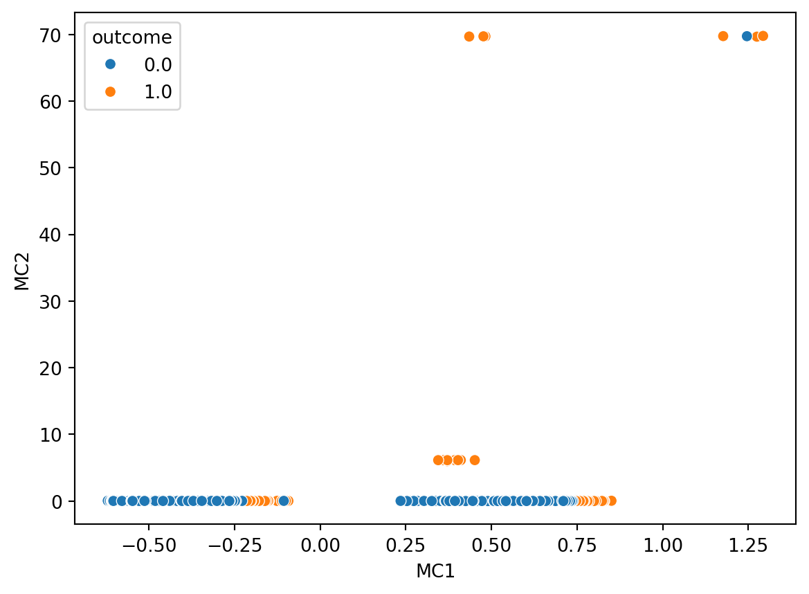
xformNd_nr.to_csv('../data/mcaNd-npc.csv',index=False)

tmp = pd.concat([out,labels],axis=1)

sns.scatterplot(
    data=tmp,
    x='MC1',y='MC2',
    hue='outcome'
)